Raw images captured by Earth observation sensors often contain geometric distortions caused by terrain variation, sensor angle, and the curvature of the Earth. These distortions mean that features on the ground aren't always represented in their true locations. This makes accurate analysis, mapping, and integration with other geospatial data difficult. Orthorectification of these images is essential to correct the distortions.
This tutorial walks through the orthorectification process using the CATALYST Professional Python API, explaining the import, GCP/TP collection and refinement processes.
The CATALYST Professional Python Cookbook provides more detailed information on various workflows, including Satellite Photogrammetry, along with sample scripts to help guide implementation.
The first step, as shown in Lines 1 to 7, is to import the necessary modules and libraries such as the built in os , sys and pathlib modules, and others related to the CATALYST Python API. The PCI algo module gives access to all the PCI functions with a single import. The following modules were also imported from the Python API
cts module - contains classes with information about the coordinate systems and transformations of the data.datasource module - handles the reading and writing of datasets as well as holds classes with metadata, CRS, and other informationpath module - has functions, such as find_files_by_masks(), which searches input sources for files.inputsource module - allows functions to iterate over data sources, such as in mfiles.import os
import sys
from pathlib import Path
from pci import algo
from pci import get_global_dem_filename
from pci.api import cts, datasource as ds
from pci.api.path import find_files_by_masks
from pci.api.inputsource import MFileSource
The next set of lines initiates the directory variables and creates folders as needed. This tutorial uses Pleiades Neo stereo imagery as the input data.
The link file, ortho, epipolar, and dem folders are created within the output folder to hold their appropriate files (which will be explained further in the script). The ref_image variable contains the reference image used to collect the GCPs, along with the global elevation model found in the dem variable. This DEM variable is the path to the gmted2010.pix file that comes with the CATALYST Professional installation - C:\PCI Geomatics\CATALYST Professional\etc.
An mfile is also specified. This text file will hold the paths and parameters required for the functions in this script. Learn more about MFILEs on the CATALYST Profession Help Documentation - Using An MFILE With A CATALYST Professional Algorithm.
# OUTLINE FOLDERS & PATHS
indir = r"H:\Tutorials\Python Orthorectification\data"
outdir = r"H:\Tutorials\Python Orthorectification\output"
if not os.path.exists(outdir):
os.mkdir(outdir)
# link file folder
links_dir = r"H:\Tutorials\Python Orthorectification\output\links"
if not os.path.exists(links_dir):
os.mkdir(links_dir)
# ortho images folder
ortho_dir = os.path.join(outdir, "orthos")
if not os.path.exists(ortho_dir):
os.mkdir(ortho_dir)
# epipolar images folder
epi_dir = os.path.join(outdir, "epipolars")
if not os.path.exists(epi_dir):
os.mkdir(epi_dir)
# dem output folder
dems_dir = os.path.join(outdir, "dems")
if not os.path.exists(dems_dir):
os.mkdir(dems_dir)
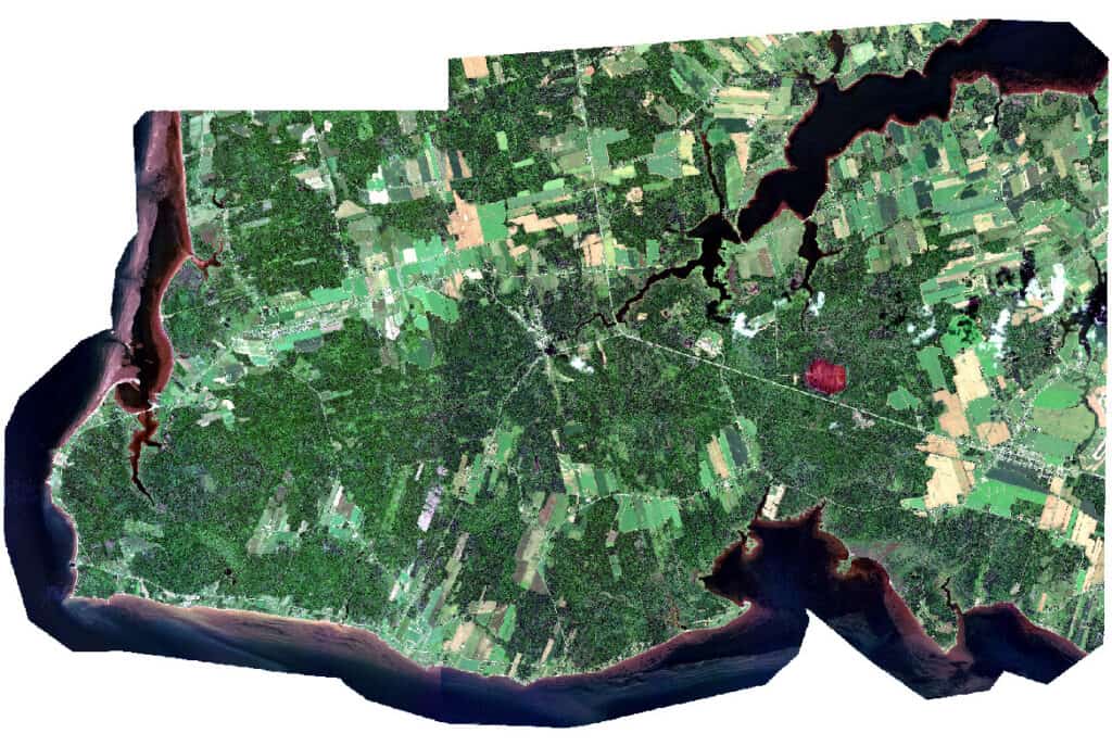
ref_image = os.path.join(indir, "Ref\s5_06406_4634_20061017_p10_1_utm20.tif")
dem = get_global_dem_filename()
mfile = os.path.join(outdir, "input.mfile")
The input data is found using the find_files_by_masks() function from the API. This function recursively searches the input folder for files matching the search pattern DIM_*_MS*.xml representing the multispectral key file. The file paths are then added to the infiles list. This list is iterated over to apply various functions to each input file that was found. One of these functions is the LINK algorithm, which is used to create a live PCIDSK link file to the input imagery. This preserves the integrity of the source file by creating indirect access to the imagery.
# Find all input key files
infiles = find_files_by_masks(indir, 'DIM_*_MS*.xml')
for filename in infiles:
# Create Link files
link_file = os.path.join(links_dir, Path(filename).stem + ".pix")
algo.link(fili=filename, filo=link_file)
The next step in the orthorectification process is the collection of Ground Control Points (GCPs) to improve the accuracy of the model by aligning the images to known ground coordinates. The AUTOGCP algorithm is used for this, with the following parameters:
dbic = [1] -> input image channel. In this dataset, channel one is the Red band.fileref -> input reference image file.filedem -> input DEM file.searchr = [50] -> search radius.The output of this algorithm is the GCP segment number, where a segment value of [-1] signifies that no GCP segments were created. This value is entered into the gcp_seg variable.
# Collect GCPs
gcp_seg = algo.autogcp(mfile=link_file, dbic=[1], filref=ref_image, filedem=dem, searchr=[50])With each successful collection, the GCPs are refined to remove the points with large residual errors. This is done using the GCPREFN algorithm with the following parameters:
mfile - the link file.dbgc - the input GCP segment, which was obtained from the GCP collection output.modeltyp = 'RF' -> the model type used for refining the GCPs. The Rational Function model was used.order = [0] -> the polynomial transformation order number for the model.reject = [5,1,1] -> the method with which the GCPs will be rejected. The first item determines the rejection mode, where 5 represents the RMS error of points to reject. The other two items represent the threshold for the x/y RMS values. The x-RMS and y-RMS values higher than 1 are rejected. # Refine GCPs
if gcp_seg != [-1]:
algo.gcprefn(file=link_file, dbgc=gcp_seg, modeltyp="RF", order=[0], reject=[5,1,1])
In addition to the GCP refinement, the file paths with successful GCPs are added to the mfile, along with their GCP segment (separated by a semi-colon). This allows easy reading from other algorithms that require these values. Files for which GCPs could not be collected are skipped and excluded from the mfile, with a message printed to the terminal indicating this.
# Add files to mfile
with open(mfile, "a") as f:
f.write(f"{link_file};{gcp_seg}\n")
else:
print(f"Couldn't collect GCPs for image: {link_file}")
The MFileSource class holds the mfile. This class is checked to ensure there are files to be processed. If there aren't, the script prints a message and exits.
Tie Points (TPs) are also essential in improving the model by aligning the images to each other. This helps to apply GCPs to areas in an image where there aren't any.
To start, the coordinate system information is extracted from an image using the Dataset class' crs property (using open_dataset()). This property is then stripped to extract the mapunits, with the cts module's crs_to_mapunits() function. This is used in the creation of the OrthoEngine project. The CRPROJ algorithm is used to create an OrthoEngine project with the input images. The Rational Functions model is used for this project (in modeltyp), where the model is extracted from the input images using the 1st order RPC adjustment - RFI1.
mfilesource = MFileSource(mfile)
if not mfilesource.is_empty():
# Extract mapunits
projection = ds.open_dataset(infiles[0]).crs
mapunits = cts.crs_to_mapunits(projection)
# Create OrthoEngine Project, which is required for the bundle adjustment
proj = os.path.join(outdir, "import_oemodel.prj")
algo.crproj(mfile=mfile, oeproj=proj, modeltyp="RFI1", mapunits=mapunits)
<CODE FOR ALGORITHMS>
else:
print("No input files found")
sys.exit()
Once the OE project has been created, AUTOTIE is run with the new project and the input DEM to collect the TPs, and is output to another OE project (tp_oeproj)
# Run Automatic Tie Point Collection
tp_oeproj = os.path.join(outdir, "output_oetp.prj")
algo.autotie(mfile=proj, oeprojo=tp_oeproj, filedem=dem)
# Run automatic Tie Point Refinement
algo.tprefn(oeproji=tp_oeproj, reject=[5, 0.5, 0.5])
# Calculate the mathematical model from GCPs (rational function model) required to orthorectify the imagery
algo.rfmodel(mfile=mfile, numcoeff=[3])
Although there is an existing DEM that can be used to orthorectify the imagery, since stereo data is used in this workflow, a DEM can be extracted from the input imagery and used to orthorectify it. This ensures sensor-consistency, temporal alignment, and reduces positional offsets while providing relative accuracy. Since the model for the imagery has already been computed and improved with GCPs and TPs, the next stem in the process is generating epipolar pairs. The EPIPOLAR algorithm is used to do this with the MAX pair selection method (selmthd). This method uses the image with the highest amount of overlap to generate a stereo-pair for each image. Once the epipolar pairs have been generated, a geocoded dem can be extracted from them using AUTODEM. Since the output of this algorithm is a Digital Surface Model (DSM), it can be further filtered into a Digital Terrain Model using the DSM2DTM algorithm.
For more detailed information on the DEM Extraction process, visit our Tutorials webpage.
# Generate the epipolar images, which are used to triangulate the 3D coordinates for the DEM
algo.epipolar(mfile=links_dir, dbic=[3], selmthd="max", sampling=[1], outdir=epi_dir)
# Automatically extract a Digital Surface Model from satellite stereo pairs
geocoded_dsm = os.path.join(dems_dir, "geocoded_dsm.pix")
algo.autodem(mfile=epi_dir, outdir=dems_dir, filedem=geocoded_dsm, pxszout=[6,6])
# convert DSM to DEM (Automatically remove surface features such as trees and buildings from DSM)
dtm = os.path.join(dems_dir, "dem.pix")
algo.dsm2dtm(fili=geocoded_dsm, dbic=[1], filo=dtm, dboc=[1], objsize=[150], gthresh=[35], tertype="hilly",
bumpflt=[9,5,9,5], pitflt=[7,5], medflt=[9])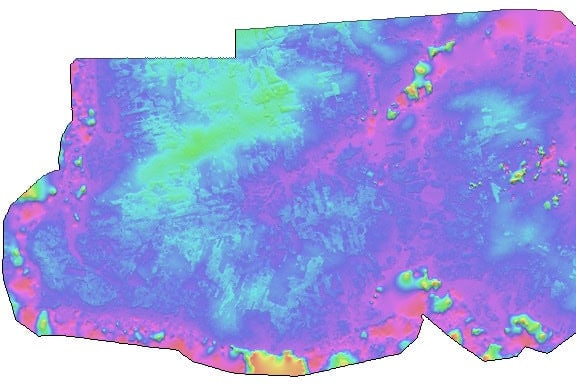
Finally, the images can be orthorectified with the improved model and new DTM. CATALYST Professional's ORTHO algorithm uses geometric models to orthorectify images with the output horizontal (bxpxsz) and vertical (bypxsz) pixel sizes as 4 each.
# Orthorectify the imagery with the new and improved math model (RPC segment) and extracted dem
algo.ortho(mfile=links_dir, filo=ortho_dir, ftype="pix",
bxpxsz="4", bypxsz="4", filedem=dtm)
import os
import sys
from pathlib import Path
from pci import algo
from pci import get_global_dem_filename
from pci.api import cts, datasource as ds
from pci.api.path import find_files_by_masks
from pci.api.inputsource import MFileSource
# Outline folders and paths
indir = r"H:\Tutorials\Python Orthorectification\input_data"
outdir = r"H:\Tutorials\Python Orthorectification\output"
if not os.path.exists(outdir):
os.mkdir(outdir)
# Link file folder
links_dir = r"H:\Tutorials\Python Orthorectification\output\links"
if not os.path.exists(links_dir):
os.mkdir(links_dir)
# Ortho images folder
ortho_dir = os.path.join(outdir, "orthos")
if not os.path.exists(ortho_dir):
os.mkdir(ortho_dir)
# Epipolar images folder
epi_dir = os.path.join(outdir, "epipolars")
if not os.path.exists(epi_dir):
os.mkdir(epi_dir)
# DEM output folder
dems_dir = os.path.join(outdir, "dems")
if not os.path.exists(dems_dir):
os.mkdir(dems_dir)
ref_image = os.path.join(indir, "Ref\s5_06406_4634_20061017_p10_1_utm20.tif")
dem = get_global_dem_filename()
mfile = os.path.join(outdir, "input.mfile")
# Find all input key files
infiles = find_files_by_masks(indir, 'DIM_*_MS*.xml')

for filename in infiles:
    # Create Link files
    link_file = os.path.join(links_dir, Path(filename).stem + ".pix")
    algo.link(fili=filename, filo=link_file)
    # Collect GCPs
    gcp_seg = algo.autogcp(mfile=link_file, dbic=[1], filref=ref_image, filedem=dem, searchr=[50])
    # Refine GCPs
    if gcp_seg != [-1]:
        algo.gcprefn(file=link_file, dbgc=gcp_seg, modeltyp="RF", order=[0], reject=[5,1,1])
        # Add files to mfile
        with open(mfile, "a") as f:
            f.write(f"{link_file};{gcp_seg}\n")
    else:
        print(f"Couldn't collect GCPs for image: {link_file}")
mfilesource = MFileSource(mfile)
if not mfilesource.is_empty():
# Extract mapunits
projection = ds.open_dataset(infiles[0]).crs
mapunits = cts.crs_to_mapunits(projection)
# Create OrthoEngine Project, which is required for the bundle adjustment
proj = os.path.join(outdir, "import_oemodel.prj")
algo.crproj(mfile=mfile, oeproj=proj, modeltyp="RFI1", mapunits=mapunits)
# Run Automatic Tie Point Collection
tp_oeproj = os.path.join(outdir, "output_oetp.prj")
algo.autotie(mfile=proj, oeprojo=tp_oeproj, filedem=dem)
# Run automatic Tie Point Refinement
algo.tprefn(oeproji=tp_oeproj, reject=[5, 0.5, 0.5])
# Calculate the mathematical model from GCPs (rational function model) required to orthorectify the imagery
algo.rfmodel(mfile=mfile, numcoeff=[3])
# Generate the epipolar images, which are used to triangulate the 3D coordinates for the DEM
algo.epipolar(mfile=links_dir, dbic=[3], selmthd="max", sampling=[1], outdir=epi_dir)
# Automatically extract a Digital Surface Model from satellite stereo pairs
geocoded_dsm = os.path.join(dems_dir, "geocoded_dsm.pix")
algo.autodem(mfile=epi_dir, outdir=dems_dir, filedem=geocoded_dsm, pxszout=[6,6])
# Convert DSM to DEM (Automatically remove surface features such as trees and buildings from DSM)
dtm = os.path.join(dems_dir, "dem.pix")
algo.dsm2dtm(fili=geocoded_dsm, dbic=[1], filo=dtm, dboc=[1],
objsize=[150], gthresh=[35], tertype="hilly",
bumpflt=[9,5,9,5], pitflt=[7,5], medflt=[9])
    # Orthorectify the imagery with the new and improved math model (RPC segment) and extracted dem
    algo.ortho(mfile=links_dir, filo=ortho_dir, ftype="pix",
               bxpxsz="4", bypxsz="4", filedem=dtm)
else:
print("No input files found")
sys.exit()