DEM Extraction – Satellite

INTRODUCTION

The following is a step-by-step tutorial of the procedure for extracting a digital surface model (DSM) (also referred to as a digital elevation model, or DEM) from stereo imagery and converting it to a digital terrain model (DTM). A DSM represents the earth’s surface and includes all objects on it, e.g., buildings, trees, etc. Many applications, however, such as orthorectification workflows, require a DTM as the preferred product. DTMs only include the elevation of ‘bare earth’ with vegetation, buildings and other man-made features removed (though roads and bridges are typically retained). As conversion from a DSM to a DTM through manual editing can be a very time-consuming process, CATALYST Professional has automated the DSM to DTM conversion.

This workflow can be used for DEM extraction from any supported stereo optical satellite data.

More information on each of the steps that are run in this tutorial is included in the online Help Documentation for CATALYST Professional.

THE DEMO DATA

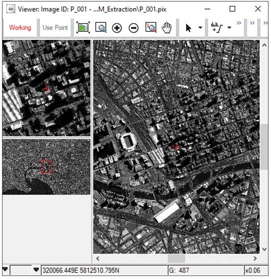
In this tutorial, sample Pléiades 1A imagery over Melbourne, Australia is used. The imagery, called the Pléiades Primary Tristereo Bundle, is a primary data set consisting of panchromatic (PAN), multispectral (MS), PMS and tri-stereoscopy images of Melbourne, Australia. The dataset is available for download from Airbus Defense and Space.

A great innovation of the Pléiades system is to offer high-resolution stereoscopic coverage. The stereoscopic coverage is realized by only a single flyby of the area, which enables collection of a homogeneous product quickly. In addition to the “classical” forward and backward looking stereoscopic imaging, Pléiades can acquire an additional quasi-vertical image (tri-stereoscopy), thus enabling the user to have an image and its stereoscopic environment (see below).

Forward and backward scans:

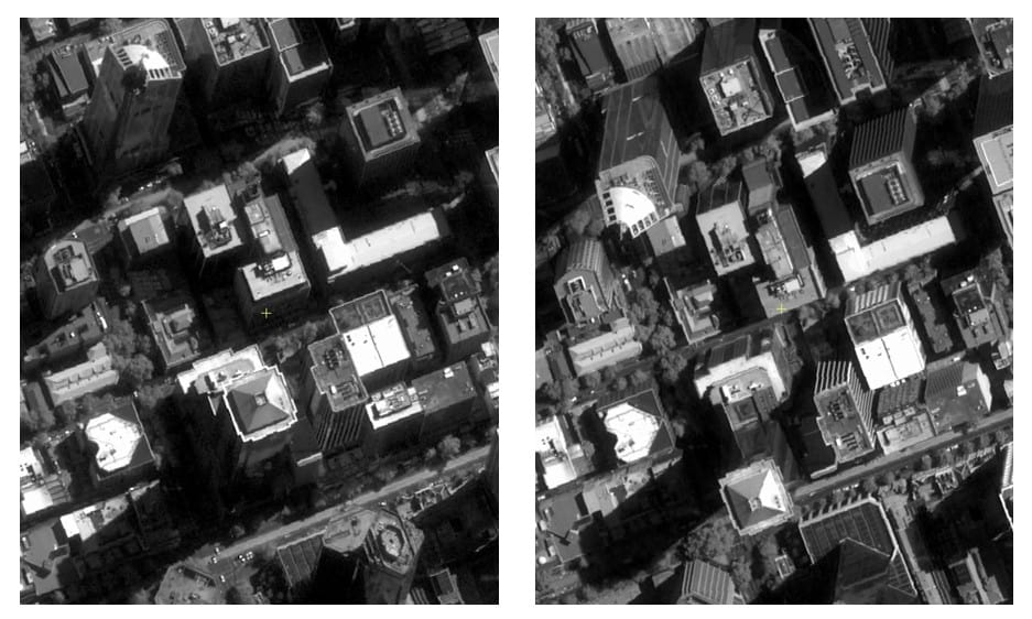
Tri-stereoscopic scan:

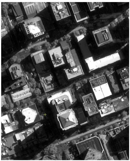
In general, a forward- and backward-looking stereo pair produces the highest accuracy, but this combination’s use is limited to areas with gentle terrain. A nadir and forward/backward looking stereo pair can be used in most types of terrain.

1. Project setup and data ingest

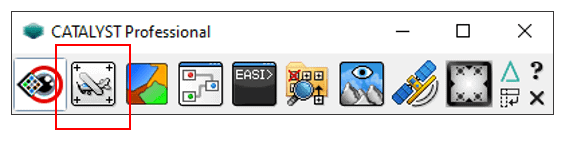
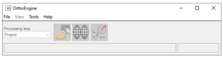
To begin, you will need to create an OrthoEngine project, choose the appropriate math model, and add your imagery.

1.1. Creating the project

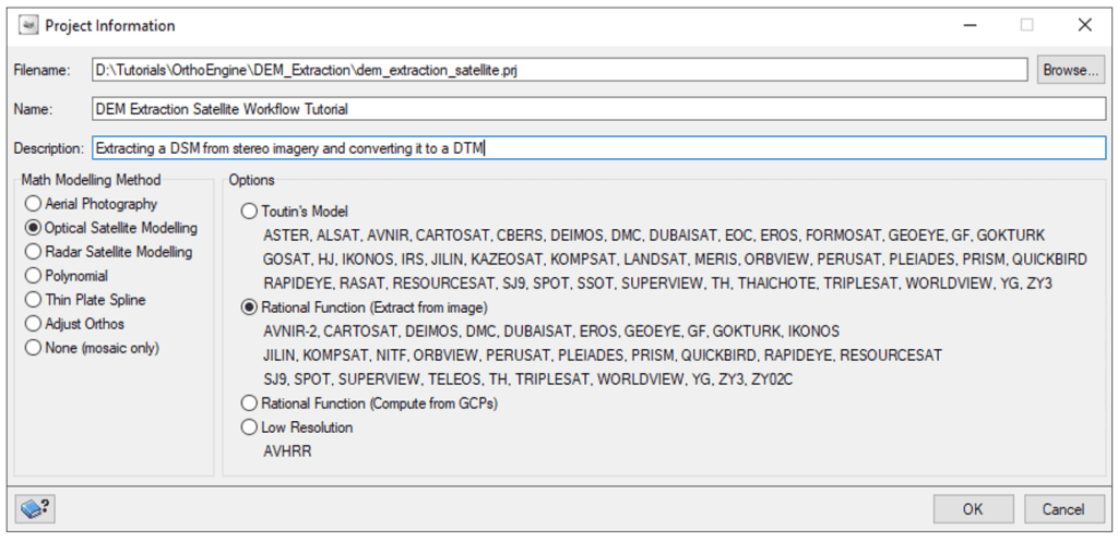
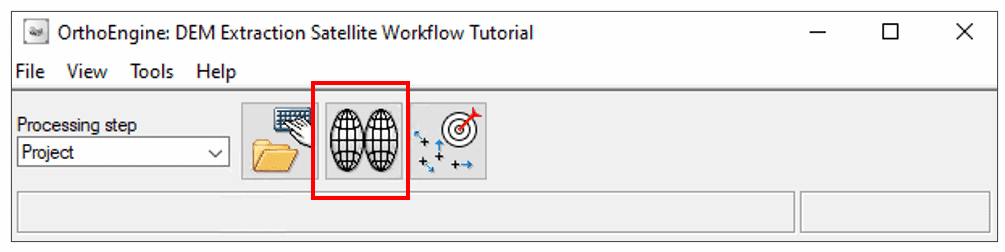
To create a new OrthoEngine project:

1. Open OrthoEngine from the CATALYST Professional toolbar.
   
2. The OrthoEngine toolbar opens. Navigate to File > New.
   
3. The Project Information window opens.
   • Give your project a Filename, Name and Description.
   • Under Math Modeling Method, select Optical Satellite Modelling.
   • Under Options, select Rational Function (Extract from image).

OPTIONS FOR MODELLING

Toutin’s Model – A rigorous model that compensates for known distortions to calculate position and orientation of the sensor at time of image acquisition. Suitable for use with any optical satellite data, regardless of resolution, such as CARTOSAT, LANDSAT, or SPOT.

Rational Function (Extract from image) and Rational Function (Compute from GCPs) – Simple math models that builds correlations between pixels and ground locations. They can be applied to any image dataset. Use this math model in the following situations:

• The sensor model is proprietary (classified).
• The image has been processed geometrically.
• The data provider computed the math model and distributed it with the image.
• You do not have the whole image.
• Information needed for a rigorous math model, e.g., the orbital segment containing the viewing geometry which generates the rational polynomial coefficients (RPCs), is missing.
  • To import the RPCs from a file, select Rational Function (Extract from image).
  • When the RPCs are calculated based on the GCPs that you collect, select Rational Function (Compute from GCPs).

 Low Resolution – For use with advanced very-high-resolution radiometer (AVHRR) data.

For more information on choosing a math model, click on the CATALYST Help button or search Creating a project and selecting a math model in the CATALYST Help.

4. Click OK.

Note: At this point, it’s a good idea to save the project via File > Save. This saves your progress to the OrthoEngine project (.PRJ) file.

1.2. Adding the imagery

Check the CATALYST Sensor Support page to see if your sensor data is supported.

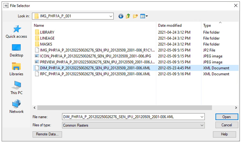
Note: Search the sensor name of your imagery in CATALYST Help to determine which key file type to use to open the image. the key file name for Pléiades is DIM_PHR1A_*.xml.

The data to input will be:

• a back scan image (file name: DIM_PHR1A_P_201202250026276_SEN_IPU_ 20120509_2001-006.XML) and
• a forward scan image (file name: DIM_PHR1A_P_201202250025329_SEN_IPU_ 20120509_2001-008.XML).

To view the images, open them in Focus. They should look like the images shown in the Demo Data section.

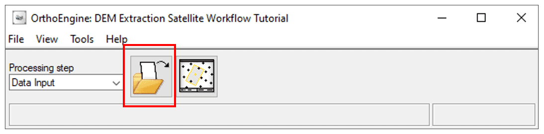
To add imagery:

1. On the OrthoEngine toolbar > Processing Step > Choose Data Input.
2. Click the Open a new or existing image button.
   
3. The Open Image window opens. Click Add Image.
4. From the File Selector window, navigate to the folder containing your first image file.
   • For the tutorial dataset we open the folder for image IMG_PHR1A_P_001.
5. Select the sensor’s key file from the folder.
   • For Pléiades data, select the DIM_PHR1A_*.xml file: DIM_PHR1A_P_201202250026276_SEN_IPU_ 20120509_2001-006.XML.
     
6. A question window appears, reading Do you want to import data file to PIX file to optimize processing? Click Yes.
7. A File Selector window opens. Type a File name for the PIX file output, e.g. P_001.pix.
8. Click Save.
9. A question window appears, reading Do you wish to create overviews now? Click Yes.
10. Your new PIX file now appears in the Open Image window.
11. Repeat Steps 3-10 for your second image, for this tutorial: IMG_PHR1A_P_003. The Open Image window now lists both uncorrected images.
    
12. At this point, you can choose to view the PIX images:
    • Select an image from the Open Image window and click Open. The Collection Viewer window opens, displaying the image in zoom view, overview view, and main view (at one-to-one resolution).
      
    • For more information on using the Collection Viewer, search Collection Viewer in CATALYST Help.
    • Close out of the viewer.
13. On the Open Image window, click Close.

1.3. Setting output projection

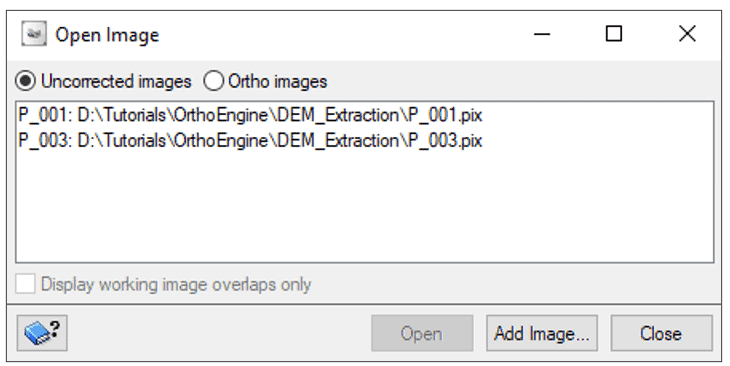
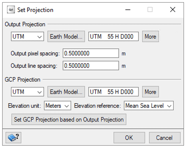
You do not need to set the projection; that is, the output projection and resolution will be set automatically from the first image you have added to your project.

If the Set Projection window pops up after completing the Project Information window, click Cancel to leave the automatically-chosen projections and close the window.

1. To view/change your projection:
   On the OrthoEngine toolbar > Processing Step > Choose Project.
2. Click the Set output and GCP projection button.
   
3. The Set Projection window opens.
   
4. If desired, change the projection of the output images or GCPs. For this tutorial, we leave them the same as the input projection (filled automatically).
5. Click OK.
6. For more information on projections, click on the CATALYST Help button or search Setting the Projection in CATALYST Help.

2. GCP/TP Collection (Optional)

You can optionally choose to collect GCPs and TPs for your project to improve the math model. More information on how to collect GCPs and TPs is outlined in the Optical Satellite Orthorectification tutorial.

For DEM extraction, you want to ensure that the stereo images are very well aligned to each other to ensure the highest quality DEM. Therefore it is highly recommended to collect TPs to improve relative accuracy.

3. DEM Extraction

OrthoEngine uses image correlation to extract matching pixels in the two images and then uses the sensor geometry from the computed math model to calculate x, y, and z positions of the DEM. Creating epipolar images increases the speed of the correlation process and reduces the possibility of incorrect matches.

3.1. Creating an epipolar image

Epipolar images are stereo pairs that are reprojected so that the left and right images have a common orientation, and matching features between the images appear along a common x-axis. For details, search Understanding epipolar images in CATALYST Help.

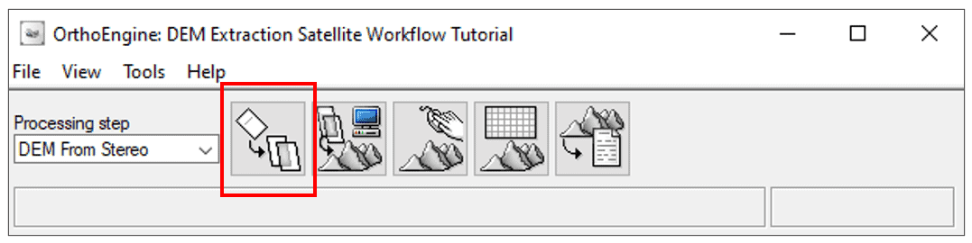
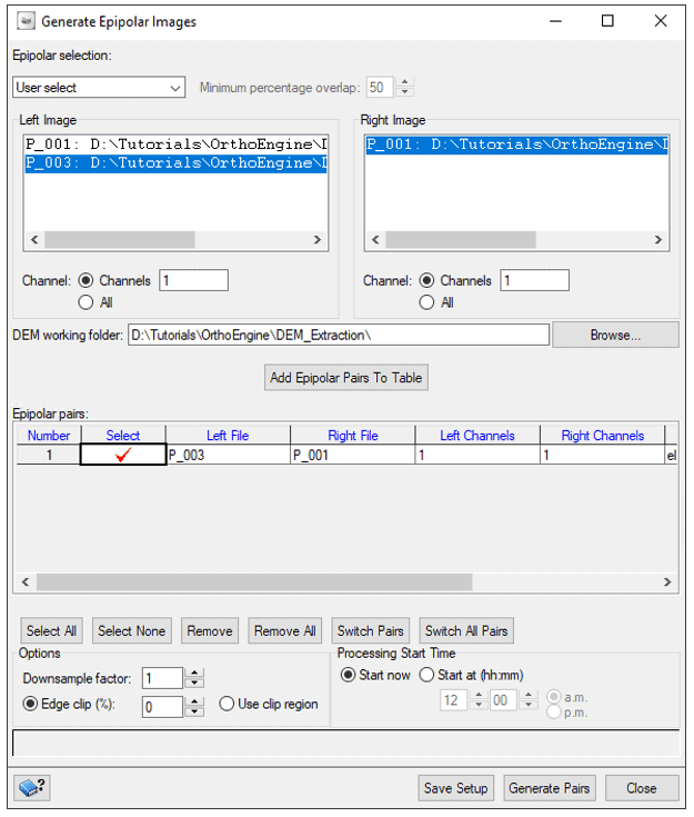
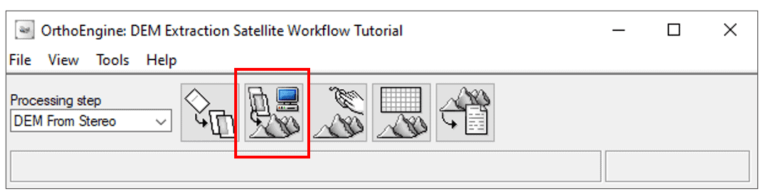
To create an epipolar image:

1. On the OrthoEngine toolbar > Processing Step > Choose DEM From Stereo.
2. Click the Create Epipolar Image button.
   
3. The Generate Epipolar Images window opens:
   • Choose the left and right image.

Note: The concepts of left and right are used by convention; however, it is only relevant when the images are actually left and right. With some pairs, such as tristereo satellite imagery, you can use any combination of nadir, forward, and backward pairs. Typically, the left image is the most nadir (vertical-looking) image, and creates a DSM with less ‘lean’. The output DSM is created automatically with the same epipolar geometry as the image specified for the left image

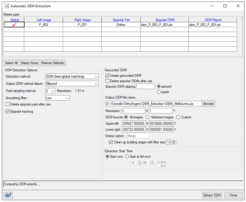
• With both images selected, click the Add Epipolar Pairs To Table button.
  

4. Click Generate Pairs.
5. Once comple/spaceted, a pop-up message states Epipolar pairs completed successfully. Click OK.
6. Close the Generate Epipolar Images window.

3.2. Generating a DEM

To generate a DEM:

1. On the OrthoEngine toolbar > Processing Step > Choose DEM From Stereo.
2. Click the Extract DEM automatically button.
   
3. The Automatic DEM Extraction window opens:
   • Select the epipolar stereo pair by clicking the Select box associated with the record.
   • Under DEM Extraction Options:
     1. For Extraction method, select SGM (Semi-global matching).
     2. For Ouput DEM vertical datum, leave as Ellipsoid. By default for Rational Functions projects, this is set to Ellipsoid. You can change the output vertical datum to MSL if you prefer.
     3. Select a Pixel sampling interval of 2.
     4. Check Epipolar tracking.
   • Under Geocoded DEM:
     1. Check Create Geocoded DEM.
     2. Navigate to your output folder and choose an output file name.
     3. For Resolution, set X and Y to 1 meter.
     4. For Output option, Merge is chosen. Leave Clean up building edges with filter size checked, with default value of 13.

OPTIONS FOR DEM EXTRACTION AND GEOCODED DEM

Extraction method –

1. SGM (Semi-global matching): Based on newer technology. Produces higher-resolution results with fewer errors and higher detail; Longer processing time.
2. NCC (Normalized cross-correlation): Lower-resolution results; Faster processing time. If lower-resolution DEMs are adequate for the project, choose the NCC method.

Epipolar tracking – The quality of the DEM is highly dependent on accurate alignment of the epipolar lines between stereo images. Errors in epipolar alignment can vary across a stereo pair, resulting in a DEM with large patches of poor quality elevation values. This is especially true when DEMs are generated at full resolution. Errors can occur even if the epipolar lines are shifted by a single line. This option enables tracking of changes in the epipolar line over the stereo pair and can automatically compensate for small gradual errors. Epipolar tracking increases processing time (typically 20-30%) and there is a small possibility of introducing errors in an otherwise good DSM.

Output option (under Geocoded DEM) –

1. Use last value: Uses the last value to replace pixel values in the overlapped area in the existing geocoded DEM by the pixel values of the geocoded DEM added to the file.
2. Average: Replaces pixel values in the overlapped area by the average pixel values between the existing geocoded DEM and the one added to the file.
3. Highest score: Uses the highest score to replace pixel values in the overlapped area by the pixel value with the highest correlation score between the existing geocoded DEM and the one added to the file.
4. Blending: Uses the mosaicking method to mosaic the DEMs by blending.
5. Merge: Merges a set of geocoded DEMs from a stereo airphoto or satellite project into a single DEM (default option for SGM extraction only). The merged DEM is typically higher quality because areas of occlusion in one DEM can be filled from another DEM. In addition, multiple DEM elevations of the same ground pixel can be used to detect blunders and increase vertical accuracy. Merge will also straighten building edges, when applicable. That is, with Merge selected, you can select the Clean up building edges with filter size check box, and type or select filter size in the field to the right. The recommended value is 13.

For more information on choosing parameters for DEM extraction and geocoded DEM, click on the CATALYST Help button or search Extracting a digital elevation model from epipolar pairs in the CATALYST Help.

4. Click Extract DEM.

Note: DEM creation will take a long time as these images have a high resolution. Occasionally, you may get artifacts in water bodies. This is normal as the algorithm processes the DEM using smaller tiles. These artifacts would need to be edited manually using our DEM Editing Tools.

5. Once completed, a popup message appears, reading 1 DEM(s) extracted successfully.
   
6. Click OK.

The final extracted Pléiades DEM of Melbourne, Australia:

3.3. Conversion to DTM

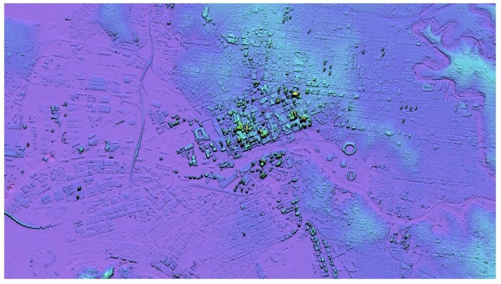
Once the DEM is extracted, you can choose to convert the DEM to a Digital Terrain Model (DTM). DTMs only includes the elevation of the ‘bare earth’ with vegetation, buildings and other man-made features removed (though roads and bridges are typically retained). A DTM is the preferred product to use in an orthorectification workflow.

For more information, see the DSM to DTM Conversion Tutorial.