Object Analyst – Batch Classification in Python

In CATALYST Professional, Object Analyst is an object-based image-analysis (OBIA) classification. It is used to segment an image into objects for classification and analysis. It differs from the traditional pixel-based approach, which focuses on a single pixel as the source of analysis.

Object Analyst algorithms can be run using the CATALYST Python API. These algorithms allow users to easily run an object-based classification on many datasets.

Introduction

The CATALYST Professional Object Analyst workflow has a batch classification feature. By using batch classification, you can run classification simultaneously on a collection of images with similar qualities of acquisition. The collection can be any aerial, satellite, or SAR imagery you want classify similarly, such as, but not limited to, airphotos (strips or individual images), stacks of historical imagery, overlapping images, or contiguous images.

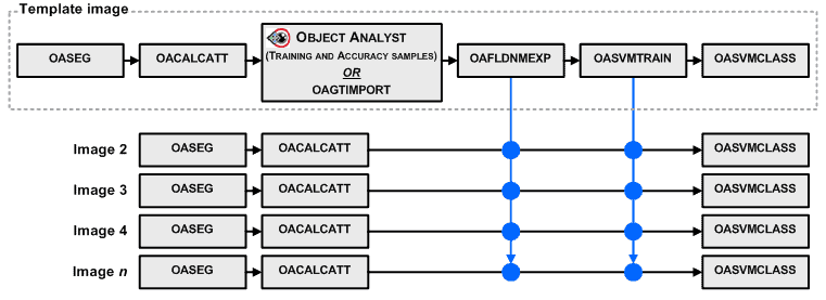
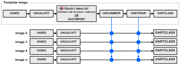
First, run a classification on an individual image that you want to use as reference image for the batch you want to process. Once the classification results from that image are deemed acceptable, then run a batch classification on the rest of the images to apply the same classification to each. The batch classification applies the following steps:

• segmentation,
• attribute calculation,
• Support Vector Machine (SVM) classification (based on the training-model file you create from the first individual image classified), and
• any number of rule-based classification steps, such as the Random Tree (RT) classification.

More information on each of the steps that are run in this tutorial is included in the online Help Documentation for CATALYST Professional.

Each of the additional images is processed in a batch Python (for this tutorial, v3.5) script, using the attribute field name text file and training model that were generated from the initial image. The diagrams below show the basic training and classification workflows for a Support Vector Machine (SVM) and a Random Tree (RT) classification.

SVM training and classification workflow 

RT training and classification workflow 

The tutorial data

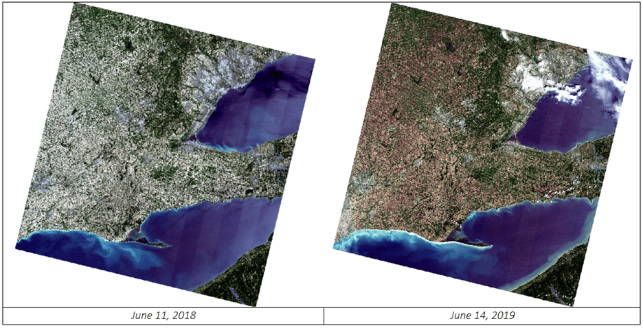
For this tutorial, multi-temporal Landsat-8 data is used, acquired in June over four different years:

1. LC08_L1TP_018030_20150603_20170226_01_T1 - June 3, 2015 (initial image)
2. LC08_L1TP_018030_20160621_20180130_01_T1 - June 21, 2016
3. LC08_L1TP_018030_20180611_20180615_01_T1 - June 11, 2018
4. LC08_L1TP_018030_20190614_20190620_01_T1 - June 14, 2019

The tutorial data can be accessed HERE.

The figures below show the datasets. Notice that two of the batch images include clouds while the initial image does not.

This factor will be part of the classification exercise. The clouds in those images will be incorrectly classified initially, as there was no cloud class in the initial image classification. After running batch classification, we will run rule-based classification on the two images with cloud to create a new cloud class.

1. Process initial image 

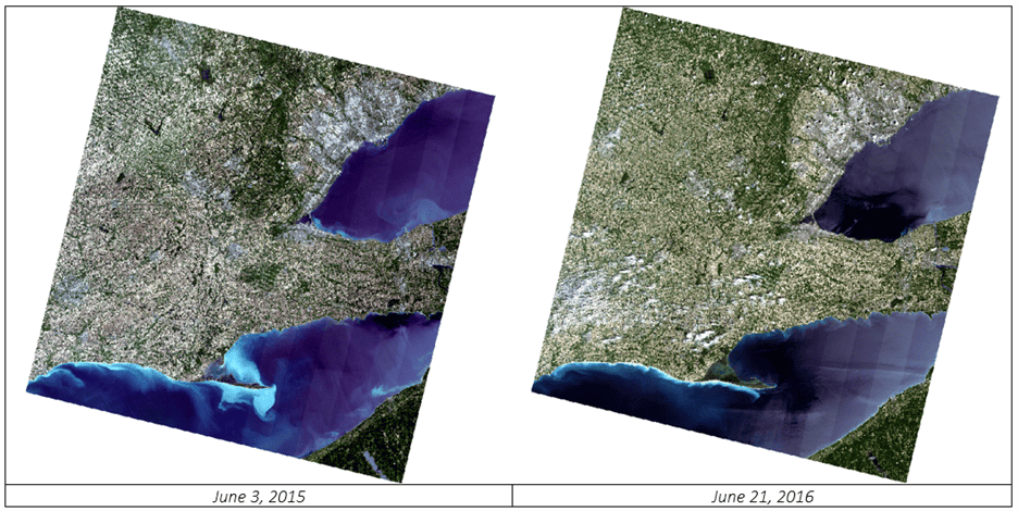
The first step is to process the initial image. In this case we will use: LC08_L1TP_018030_20150603_20170226_01_T1 (June 3, 2015) as the initial image.

The following algorithms will be run on the initial image to generate the training model and complete the classification:

• Segmentation - OASEG (OASEGSAR),
• Attribution calculation - OACALCATT (OACALCATTSAR),
• Importing ground truth - OAGTIMPORT,
• Exporting attribute fields to txt file - OAFLDNMEXP,
• Creating SVM training model - OASVMTRAIN,
• Running SVM classification - OASVMCLASS,
• Alternatively, creating and running Random Tree classification - OARTTRAIN / OARTCLASS.

You can check the CATALYST Professional Help documentation for additional information on the required parameters for each algorithm.

1.1. Import necessary modules & setup inputs/outputs 

The first step in the Python script is to import the required modules and set up the variables that will point to our input and output directories and files. You can import the following modules:

• algo: to access all the CATALYST Python API algorithms,
• os: to access the operating system’s file structure, and
• glob: to find files in a directory.

Create input and output variables as outlined below.

1.2. Segmentation - OASEG

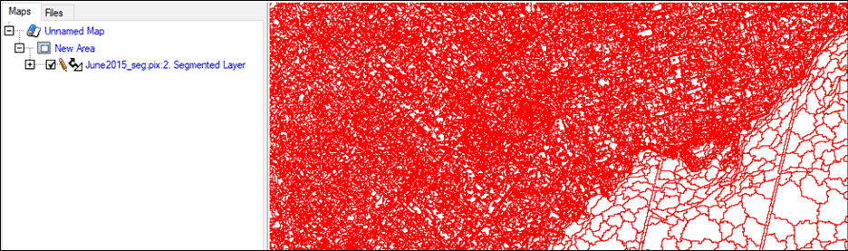
The OASEG algorithm applies a hierarchical region-growing segmentation to image data and writes the resulting objects to a vector layer. The input file (fili) is the initial image variable (init_image) that we defined above. The output image will be the new segmentation file (init_seg). The scale parameter (segscale) will be set to 35 – this will create larger segments then the default of 25.

1.3. Attribution calculation - OACALCATT

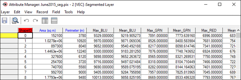
The OACALCATT algorithm calculates attributes of objects (polygons) in a vector layer, and then writes the output values to the same or a new segmentation vector layer.

The input image (fili) will be set to the initial image (image) that is being processed in the loop. Only channels 2-6 (B, G, R, NIR, SWIR) and 8 (Cirrus clouds) will be used in the attribute calculation (dbic). These attributes are calculated for each of the polygons in the segmentation layer created in OASEG (filv, dbvs). The calculated attributes are then saved back to the same segmentation layer (filo, dbov). The Maximum and Mean statistical attributes (statatt) and Rectangularity geometrical attribute (geoatt) will be calculated. Additionally, NDVI vegetation index will be calculated (index) which will help to classify vegetation.

1.4. Importing ground truth - OAGTIMPORT

The OAGTIMPORT algorithm will import a series of training or accuracy sample points into the attribute table of a segmentation file. The training or accuracy samples must be vector points (not polygons) with a field containing the class names. In this example, the ground truth dataset includes points that were collected from the initial image in Focus. You may have existing ground truth points for your own datasets.

Note: To convert existing training site or classification data from polygons to points, use the POLY2PNT algorithm.

• The point file (ground_truth) will be set as gtfili.
  • In this point file there is a field, gt_class, which lists the classification associated to this point. This field will be set for gtfldnme.
• Parameters filv, dbvs, filo and dbov will be set to the initial segmentation (init_seg) file and segment:
  • filv = Specifies the name of the file that contains existing segmentation.
  • dbvs = The number of the vector layer containing the segmentation to be updated = [2]
  • dbov = Output vector segment (overwrite) = [2]
• The samptype is set to “Training” as we want these points to generate training sites, instead of accuracy assessment sites.
• The resrule is set to “First” so the first-encountered point is used to set the training class of the segmentation polygon.

1.5. Exporting attribute fields to txt file - OAFLDNMEXP

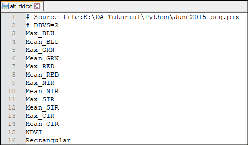
The OAFLDNMEXP algorithm exports the names of attribute fields from an OA segmentation file to a text file.

• The input file (filv) is the initial segmentation file that we created in Focus.
• The dbvs variable will be set to 2 as this is the segment number of the segmentation vector layer.
• In this tutorial we will export all attribute-field names from Object Analyst (“ALL_OA”) but fldnmflt can also be set to specific fields.
• The output text file (tfile) will be set to the fld variable that we created earlier in the script.

1.6. Creating SVM training model - OASVMTRAIN

The OASVMTRAIN algorithm uses a set of training samples and object attributes, stored in a segmentation attribute table, to create a series of hyperplanes, and then writes them to an output file containing a Support Vector Machine (SVM) training model.

• The same segmentation file that we created in Focus will be used as the input (filv).
• The field name text file (fld) will be used as another input (tfile).
• The kernel function for the SVM classification (kernel) will be the default radial-basis function (RBF).
• Finally the training model (trnmodel) parameter will be set to the training_model variable we created earlier.

1.7. Running SVM classification - OASVMCLASS

The OASVMCLASS algorithm uses the SVM method to run a supervised classification based on an SVM training model you specify. This is the final algorithm that needs to be run on the initial image in order to complete the classification. When this algorithm is run, new fields are added to the output file (filo) which include the classification information.

• The initial segmentation (filv), field name file (tfile) and training model (trnmodel) from the earlier algorithms will be used as inputs.
• The output vector file (filo) will be set to the int_seg variable and the output vector segment number (dbov) will be 2, as we want the classification fields added to the initial segmentation vector segment. This will ensure that all Object Analyst fields (i.e., attributes, training, and classification) are contained in a single vector layer.

1.8. Alternatively, running Random Tree classification - OARTTRAIN/OARTCLASS

Similar to the SVM classification algorithms you can specify the Random Trees (RT) classification algorithms, OARTTRAIN and OARTCLASS, instead. RT belongs to a class of machine learning algorithms which does ensemble classification. The classifier uses a set of object samples that are stored in a segmentation-attribute table. The attributes are used to develop a predictive model by creating a set of random decision-trees and by taking the majority vote for the predicted class.

You can choose to run the SVM algorithms or the RT algorithms. Below is code for RT algorithms.

2. Process additional images in batch

Note: See bottom of Section 2 for full Python script.

Now that the initial image is classified, we can apply that same training model to the additional images.
The first step is to create a list of all valid additional images in the add_images folder. The glob module can be used to create a list of all .pix files in the add_images folder.

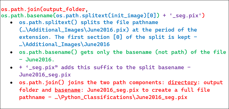
Using a for loop, iterate through the file_list. The algorithms within the loop will be run on each individual image. A new segmentation pix file (add_seg) will need to be created for each input image. The os module is used to establish the naming for the new segmentation file. The elements of the for loop are described below:

2.1. OASEG

As before, the OASEG algorithm applies a hierarchical region-growing segmentation to image data and writes the resulting objects to a vector layer.

This time, the input image (fili) will be the current image (image) that is being processed in the loop. The output image will be the new segmentation file (add_seg). The scale parameter (segscale) will once again be set to 35 to create larger segments then the default.

2.2. OACALCATT

As before, the OACALCATT algorithm calculates attributes of objects (polygons) in a vector layer, and then writes the output values to the same or a new segmentation vector layer.

The input image (fili) will be set to the current image (image) that is being processed in the loop. All other parameters and outputs are the same as for the initial attribute calculation.

2.3. OASVMCLASS or OARTCLASS

If you ran an SVM classification on the original image, we will now run the OASVMCLASS classification in a similar method to how we ran it on the initial image. The same training model and attribute field text file will be used from the initial call to OAFLDNMEXP. The current segmentation file (add_seg) will be used as both the input and output (filv/dbvs, filo/dbov).

If you ran an RT classification (OARTTRAIN and OARTCLASS) on the original image, you will use OARTCLASS for the additional images.

2.4. Python script

Once the batch processing is complete, each segmentation file will include the classification fields:

• Label – an integer class label,
• Class – a string class label, and
• Prob – a class voting probability.

You can then open the vector files in Focus and apply a representation to view the classification.

Below is the Python script for Section 2.

3. Full Python script

The full Python script for the tutorial is provided below.

4. Adjust representation of segmentation layer

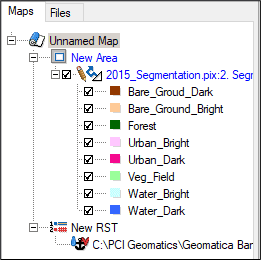
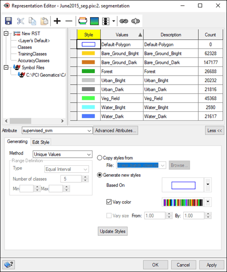
When a segmentation vector layer is loaded into Focus the classification will not be automatically shown. You will need to adjust the representation of the vector layer to show the classification. This representation can then be saved to a Representation Style Table (.RST) file and that RST file can be used to load the same representation for the additional vector layers.

4.1. Edit classification representation

To adjust the representation of the first segmentation vector file in Focus to display the classification results:

1. In Focus, open the first segmentation pix file.
   • For this tutorial, June2015_seg.pix.
2. In the Files tab, right-click the segmentation vector layer > choose View.
3. In the Maps tab, right-click the new vector layer > choose Representation Editor.
4. The Representation Editor window opens. Change the Attribute option to the Supervised Classification field.
5. Click More >>.
6. Under the Generating tab, make sure for Method that Unique Values is selected.
7. Make sure the Generate new styles option is selected and that you choose the style that you want to use.
8. Click Update Styles.
9. You can then change the colour of each class in the top section of the panel, under the Style column.

4.2. Save representation to RST file

To be able to apply the same representation to other files, you will need to first save the representation to an RST (.RST) file.

To save the representation:

1. In Focus > Maps tab > right-click new vector layer > choose Representation Editor.
2. In the Representation Editor window, click the Save button.

3. The Save As window opens. Browse to the location of your working folder and name the RST file.

4.3. Apply representation to additional vector layers

When you load the additional classifications to Focus you want to ensure that the RST file you created is linked to the map in your project. This representation can then be easily applied to the additional images.

To apply the RST to additional images:

1. In Focus > Maps tab > right-click on the Unnamed Map > Representation > choose Load.
2. Select the RST file that you just created and click Open.
3. The RST file will now be listed in the Maps tab.

4. Open the additional segmentation files in Focus.
5. In the Maps tab, right-click on one of the new vector layers > choose Representation Editor.
6. In the Representation Editor, change the Attribute drop-down menu to the SupClass field and click OK.

7. The representation from the RST file will now be applied.
8. Follow Steps 5 & 6 for each of the additional segmentation vector layers.