Details
A typical workflow starts by running the OASEG algorithm, to segment your image into a series of object polygons. Next you would calculate a set of attributes (statistical, geometrical, textural, and so on) by running the OACALCATT algorithm. Alternatively, when you are working with SAR data, you would use OASEGSAR and OACALCATTSAR. You can then, in Focus Object Analyst, manually collect or import training samples for some land-cover or land-use classes; alternatively, use OAGTIMPORT for this task. The training samples are stored in a field of the segmentation attribute table with a default name of Training.
- A segmentation with a field containing training samples
- A list of attributes
You can create the list of attributes by running OAFLDNMEXP. Alternatively, the list can be read directly from the table of segmentation attributes using field metadata that was created by OACALCATT or OACALCATTSAR.
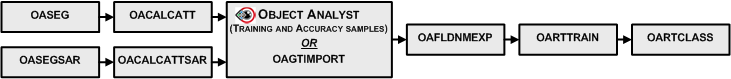
Typically, you specify as input the segmentation vector layer from OASEG or OASEGSAR.
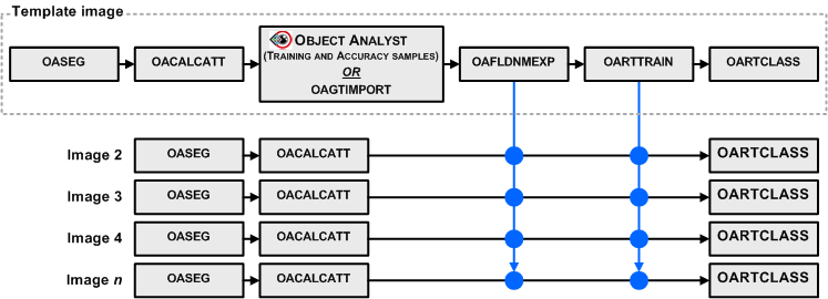
The training (OARTTRAIN) and classification (OARTCLASS) steps are distinct to allow you to reuse a trained Random Trees model for other segmentations, provided that the list of attributes is the same for all segmentations and calculated from similar images; that is, from the same sensor and in the same acquisition mode.
A single decision tree is easy to conceptualize but will typically suffer from high variance, which makes them not competitive in terms of accuracy.
One way to overcome this limitation is to produce many variants of a single decision tree by selecting every time a different subset of the same training set in the context of randomization-based ensemble methods (Breiman, 2001). Random Forest Trees (RFT) is a machine learning algorithm based on decision trees. Random Trees (RT) belong to a class of machine learning algorithms which does ensemble classification. The term ensemble implies a method which makes predictions by averaging over the predictions of several independent base models.
The Random Forest algorithm, called thereafter Random Trees for trademark reasons, was originally conceived by Breiman (2001) “as a method of combining several CART style decision trees using bagging [...] Since its introduction by Breiman (2001) the random forests framework has been extremely successful as a general-purpose classification and regression method" (Denil et al., 2014).
The fundamental principle of ensemble methods based on randomization “is to introduce random perturbations into the learning procedure in order to produce several different models from a single learning set L and then to combine the predictions of those models to form the prediction of the ensemble” (Louppe, 2014). In other words, "significant improvements in classification accuracy have resulted from growing an ensemble of trees and letting them vote for the most popular class. In order to grow these ensembles, often random vectors are generated that govern the growth of each tree in the ensemble" (Breiman, 2001).
"There are three main choices to be made when constructing a random tree. These are (1) the method for splitting the leafs, (2) the type of predictor to use in each leaf, and (3) the method for injecting randomness into the trees" (Denil et al., 2014). A common technique for introducing randomness in a Tree "is to build each tree using a bootstrapped or sub-sampled data set. In this way, each tree in the forest is trained on slightly different data, which introduces differences between the trees" (Denil et al., 2014). Randomization can also occur by randomizing "the choice of the best split at a given node... experiments show however that when noise is important, Bagging usually yield better results" (Louppe, 2014).
When optimizing a Random Trees model, “special care must be taken so that the resulting model is neither too simple nor too complex. In the former case, the model is indeed said to underfit the data, i.e., to be not flexible enough the capture the structure between X and Y. In the latter case, the model is said to overfit the data, i.e., to be too flexible and to capture isolated structures (i.e., noise) that are specific to the learning set" (Louppe, 2014).
- The minimum number of samples in a terminal node to allow it to split
- The minimum number of samples in a leaf node when the terminal node is split
- The maximum tree depth, that is, the maximum number of levels a tree can grow
- Once the Trees accuracy (defined by the Gini Impurity index) is less than a fixed threshold
- It is an excellent classifier--comparable in accuracy to support vector machines.
- It generates an internal unbiased estimate of the generalization error as the forest building progresses.
- It has an effective method for estimating missing data and maintains accuracy when up to 80% of the data are missing.
- It has a method for balancing error in unbalanced class population data sets.
- Generated forests can be saved for future use on other data.
- It gives estimates of what variables are important in the classification.
- Output is generated that gives information about the relation between the variables and the classification.
- It computes proximities between pairs of cases that can be used in clustering, locating outliers, or by scaling, give interesting views of the data.
In general, the random trees classifier, unlike the Support Vector Machine (SVM), can handle a mix of categorical and numerical variable. The Random Trees is also less sensitive to data scaling while SVM often required data to be normalized prior to the training/classification. However, SVM is reported to perform better when the training set is small or unbalanced. The Random Trees classifier is computationally less intensive than SVM and works better and faster with large training sets.
Many versions of the Random Trees algorithm exist. Object Analyst uses the OpenCV implementation which use the Gini Impurity index to determine what is a good split point for a node on the classification tree and the minimum number of samples, the maximum tree depth and the accuracy of the trees as stopping criteria. An in-depth review of the popular implementation of Random Trees is provided in Louppe (2014) at section 5.4.2.