This tutorial outlines the automatic orthorectification and mosaicking process of airphotos using Ortho-Engine. This workflow shows how to import data, automatically collect GCPs and TPs, generate orthos, and finally generate a mosaic.
The data used in this tutorial was captured using an UltraCam D camera and can be accessed from HERE.
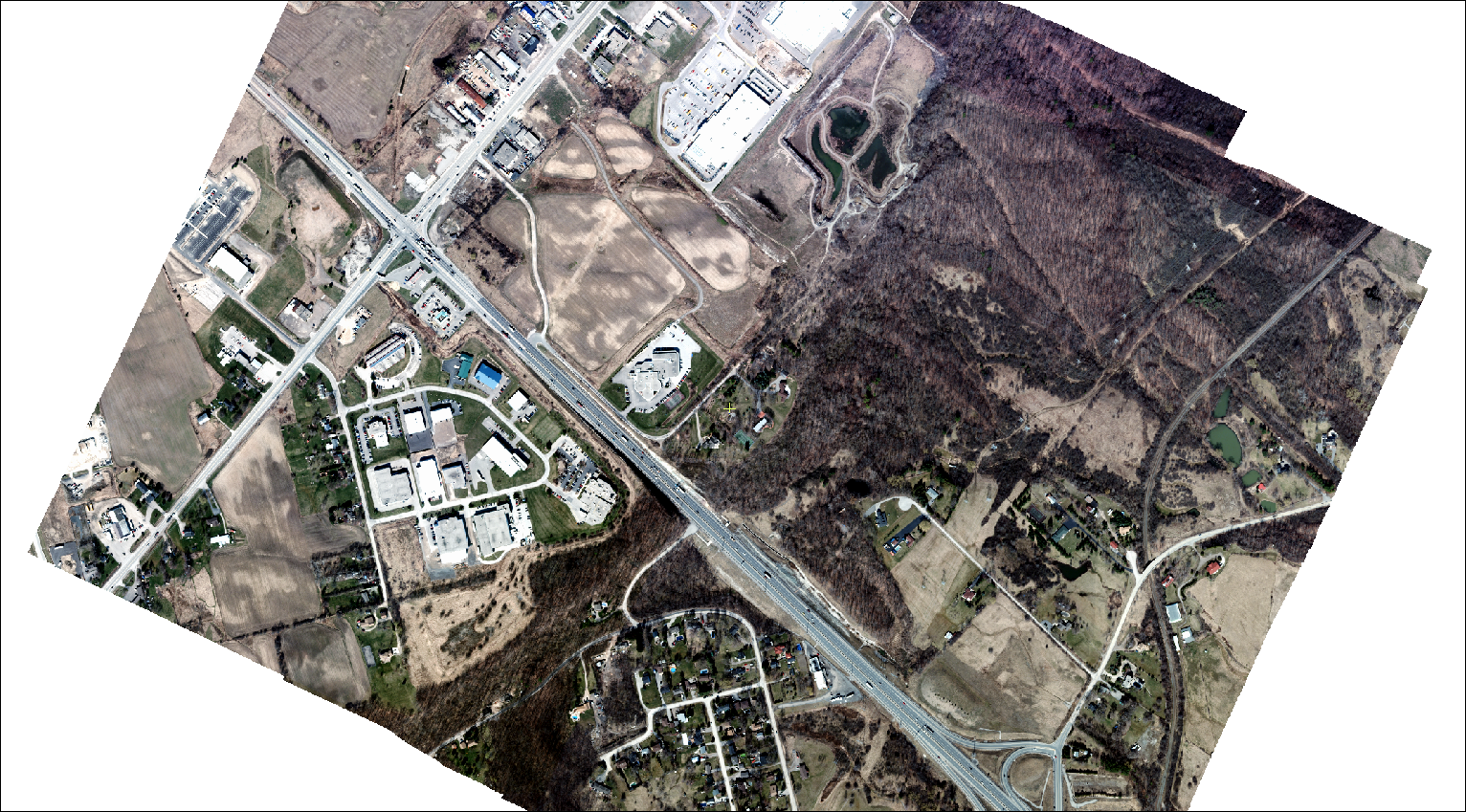
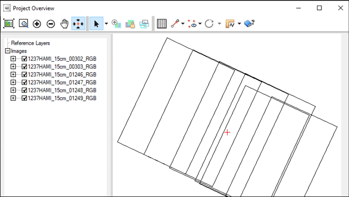
Note: When initially loading the images into Focus they appear to lie on top of each other. This tutorial explains how to process the data so that they lay in their correct geographical location.
To begin, you will need to create a new OrthoEngine project.
To set up an OrthoEngine project:
- Open OrthoEngine from CATALYST toolbar.
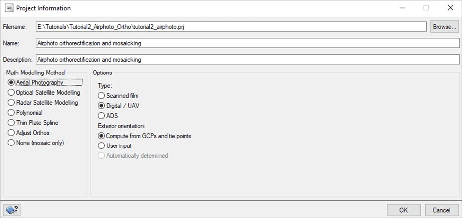
- On the OrthoEngine toolbar navigate to File > New. The Project Information window opens.
- Give your project a Filename, Name and Description. Select Aerial Photography as Math Modeling Method.
- Select Digital/UAV under Options.
- Select Compute from GCPs and tie points under Exterior orientation.
- Click OK.
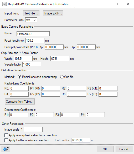
- The Digital/Video Camera-Calibration Information window opens.
- Enter the focal length, chip size and Y scale factor information.
- Click OK.
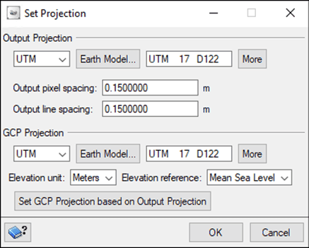
- The Set Projection window opens.
- Enter the output projection information for the images.
- Enter pixel and line spacing.
- Click OK.
- Save the project.
2. Ingesting the data
To add imagery:
- On OE toolbar, switch Processing step to Data Input.
- Click Open a new or existing image. The Open Image window opens.
- Click Add Image.
- Navigate to the location of the images, select all, and click Open.
- When prompted, choose YES to import files to PIX format. Click OK to Multiple File selection.
- The new pix files will now appear in the Open Image window.
- Close out of window.
- On the OrthoEngine toolbar click the Import exterior orientation data from text file icon.
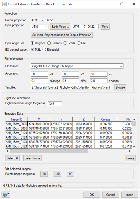
- The Import exterior orientation data from text file window opens.
- Verify Input projection, Input angle unit and EO vertical datum information.
- Enter Accuracy information, as shown below.
- For Text file, click Browse to navigate to eo.txt for the dataset. Click OK. (You will notice the GPS/INS information for the images is saved.)
- Click Import. (You will notice the GPS/INS information for the images is saved.)
- Click OK. Save.
3. Setting GCP/TP accuracy
Prior to collecting GCPs and TPs you can view and set the accuracy, or weights, of all the ground control points (GCP) and tie points (TP) in your project.
Note: Setting the proper accuracy values is very important.
- If your project consists of surveyed GCPs, accuracy entered should be sub-metre.
- For more information on setting the accuracy, go to Viewing the default accuracy values in the Help.
To set GCP/TP accuracy:
- From Processing steps, choose the Project or GCP/TP Collection step.
- Select the GCP/TP Accuracy button.
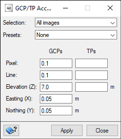
- The GCP/TP Accuracy window opens:
- Choose Selection > All Images.
- Optionally, choose a preset accuracy based on options in Presets list.
- Under GCPs and TPs, enter values by which to set accuracy of the points.
- Click Apply. The image or images are updated with the new accuracy values.
4. Collecting GCPs
Now that the images are imported, you can collect GCPs and TPs.
To collect GCPs:
- From GCP/TP Collection Processing step (which is still open), select Collect GCPs Automatically button.
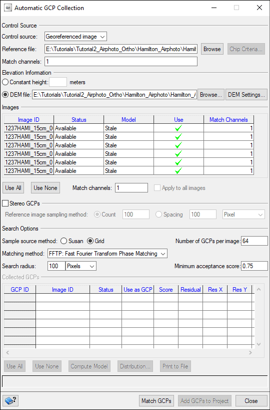
- The Automatic GCP Collection window opens:
- Change Control Source to Georeferenced image.
- For Reference file, browse to reference image. For this tutorial, Hamilton6_Mosaic.jp2.
- Under Elevation Information, click DEM file. Browse to DEM file. For this tutorial, PCI_Hamilton6_DTM_45cm.pix.
- Click OK.
- If required, adjust Search Options:
- Sample source method:
- Susan: Sample points generated automatically using corner-detection algorithm.
- Grid: Sample points generated automatically using sample points distributed evenly across overlap region.
- Matching method:
- FFTP(default): Determines shift between images using phase difference.
- NCC: Finds relative shift between two images by finding the shift that produces max cross-correlation coefficient of gray values.
- Search Radius: Define search radius around kernel.
- Min acceptance score: Enter from 0-1 which defines minimum successful match.
Note: For more details on each option in the Automatic GCP Collection window, go to Understanding automatic ground control point collection in the Help.
- Click Match GCPs.
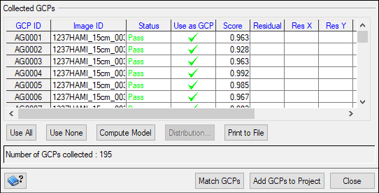
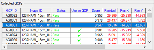
- Now, collected GCPs will be listed in the Collected GCPs panel.
- Click Compute Model to view residuals for each GCP. (If required, change Search Options and recollect GCPs.)
- Select which GCPs you would like to use. To remove a GCP from the model calculations, click on the checkmark in the column Use as GCP.
- Once you are satisfied with GCPs, click Add GCPs to Project.
- Message appears, indicating how many GCPs have been added to the project.
- You can rerun GCP collection after adding to the project to collect more GCPs.
- Close window. Save.
5. Collecting TPs
Since there are multiple images, we will collect TPs in order to further improve the model.
To collect TPs:
- From GCP/TP Collection Processing step, select Automatically collect tie points button.
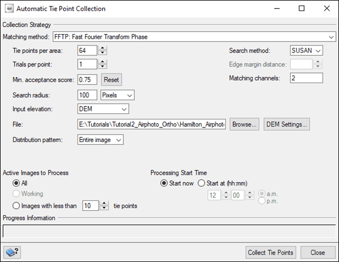
- The Automatic Tie Point Collection window opens.
- Choose Matching method. For this tutorial, choose FFTP: Fast Fourier Transform Phase.
- For Input Elevation, choose DEM.
- Browse to the DEM file. For this tutorial, PCI_Hamilton6_DTM_45cm.pix. Click OK.
Note: For more details on each option in the Automatic Tie Point Collection window, go to Understanding tie points in the Help.
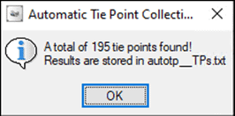
- Click Collect Tie Points.
- Algorithm executes. Once complete, a pop-up message will appear to tell you how many TPs were collected. More or less TPs will be collected based level of overlap in your dataset.
- Click OK. You can change the options and collect more TPs if required.
- Close window. Save.
6. Calculating the model
Note: Make sure to calculate the model before performing the next steps (that is, before performing the bundle adjustment).
To calculate the model:
- Go to Processing Step > Model Calculations > Compute Model.
- Save project.
- Go to GCP/TP Collection > Residual report.
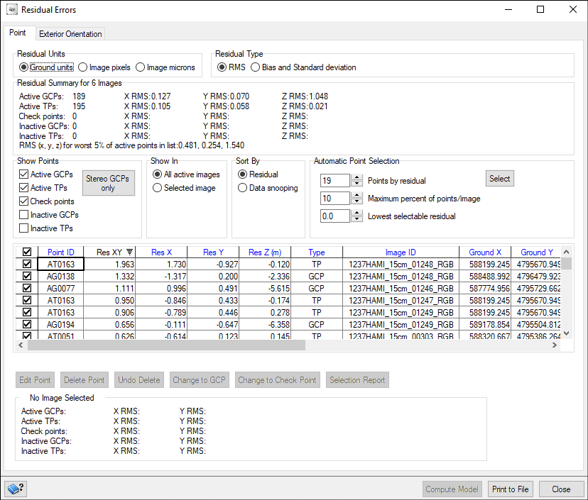
- View Residual Errors report:
- Use the report to decide if it will be necessary to conduct point thinning and refinement to achieve the accuracy according to your project’s specifications.
- Click Close.
7. Point thinning and refinement
After you have collected GCPs and TPs you can further refine them, if required. The Point Thinning and Refinement window allows you to automatically run thinning to remove redundant points and refinement to remove points with high RMS error due to poor correlation.
Note: For the subsections below, you can run them sequentially or simultaneously.
7.1. Point thinning
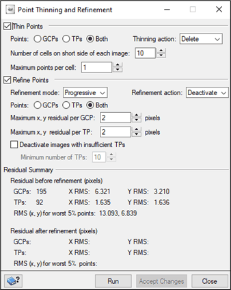
To set up point thinning, select type of points you want to thin, how you want to dispose of the points designated for removal, and then define the grid by which to divide the image into cells. By defining the grid, you can specify the how many points you want to retain in each cell.
To thin points:
- Go to Processing step > GCP/TP collection > Point thinning and refinement.
- Make sure that Thin Points box is checked off.
- Set parameters:
- Points: Select type of points you want to thin: GCPs, TPs, or Both.
- Number of cells on short side of each image: Leave as default.
- Maximum points per cell: Enter the number of points to retain in each cell (the value is used in conjunction with Number of cells on short side of each image to determine points to retain per cell).
- Thinning action: Choose to either deactivate or permanently delete the removed points.
Note: Go to Setting up point thinning in the Help for details on each parameter.
- Choose to also Refine Points or run only point thinning.
- Click Run. Click Accept changes.
7.2. Point refinement
To set up point refinement, select the type of points you want to refine, mode, how you want to dispose of the points designated for removal, and maximum x and y residual per point.
To refine points:
- Make sure that Refine Points box is checked off.
- Set parameters:
- Refinement Mode:
- Progressive: Reject points iteratively. Points with very high RMS threshold are removed. Threshold reduced iteratively based on max x and y residual specified.
- Direct: Reject points at a specific threshold. Points are rejected at precisely max x and y residual specified.
- Points: Select type of points you want to thin: GCPs, TPs, or Both.
- Maximum x, y residual per GCP/TP: Enter a value into either or both boxes depending on your points option. This value represents threshold at which to reject relevant points.
- Deactivate images with insufficient TPs: If checked, then specify threshold in the Maximum number of TPs box.
- Refinement action: Choose to either deactivate or permanently delete the removed points.
Note: Go to Setting up point refinement in the Help for details on each parameter.
- Choose to also Thin Points or run only point refining.
- Click Run. Click Accept changes.
8. Generating the residual report
The residual report helps determine if the math-model solution is good enough. Residual errors do not necessarily reflect errors in the GCPs/TPs, but rather overall quality of the math model. In other words, residual errors are not necessarily mistakes that need correcting. While they may indicate bad points, generally, they simply indicate how well the computed math model fits the ground control system.
To run residual report:
- From the GCP/TP Collection toolbar open the Residuals report icon.
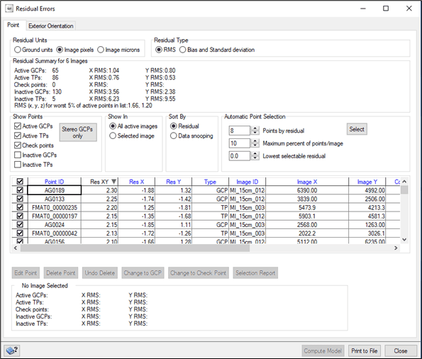
- The Residual Errors window opens. The residual information on the collected GCPs and TPs are displayed in this window.
Note: For explanations on each of the options in the Residual Errors window, go to Understanding the residual reports in the Help.
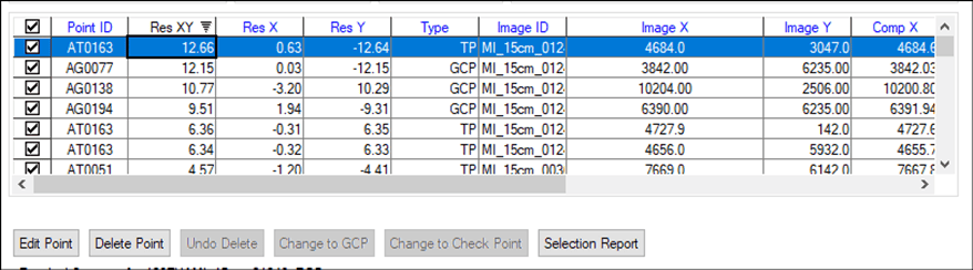
- If you have any points with very high residual errors you can remove them from the model using the Delete Point button.
- Once satisfied, click Compute Model.
- Close window. Save.
9. Performing QA on the GCP/TP distribution
To perform QA on the TP distribution:
- Go to View > Project Overview.
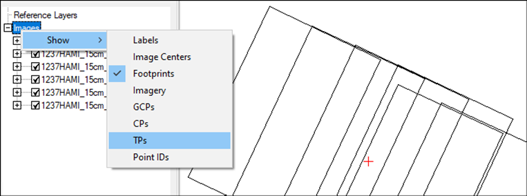
- Right-click images, select Show > TPs.
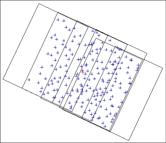
- Ensure a good distribution of TPs.
- Close window.
10. Generating ortho images
You can now generate orthorectified images.
To generate orthorectified images:
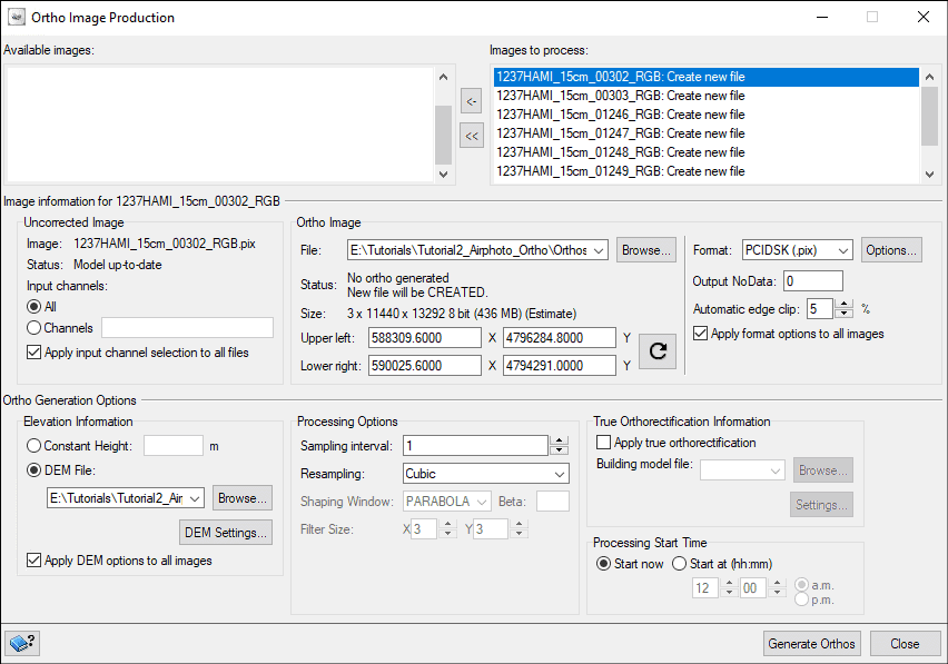
- Go to Processing step > Ortho Generation > select Schedule ortho generation.
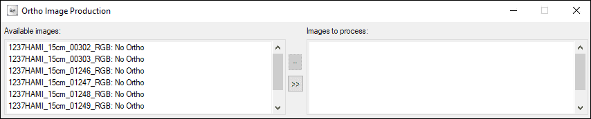
- The Ortho Image Production window opens. In the window, Available images will appear as:
- Select all images in the left panel (Available images) and add them to the right panel (Images to process).
- [In your working folder, create an output folder called Orthos.]
- For File, browse to the output location for your ortho images.
- Select DEM.
- Modify any of the default parameters to suit your data.
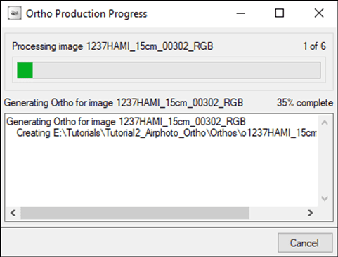
- Click Generate Orthos. Progress is displayed in the Ortho Production Progress window:
- Close window. Save.
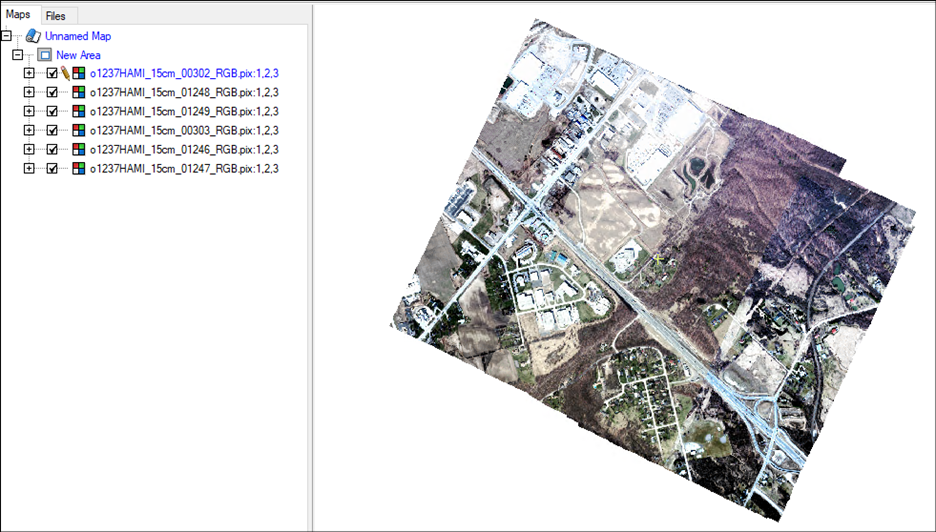
- To view the results, open the orthos in Focus:
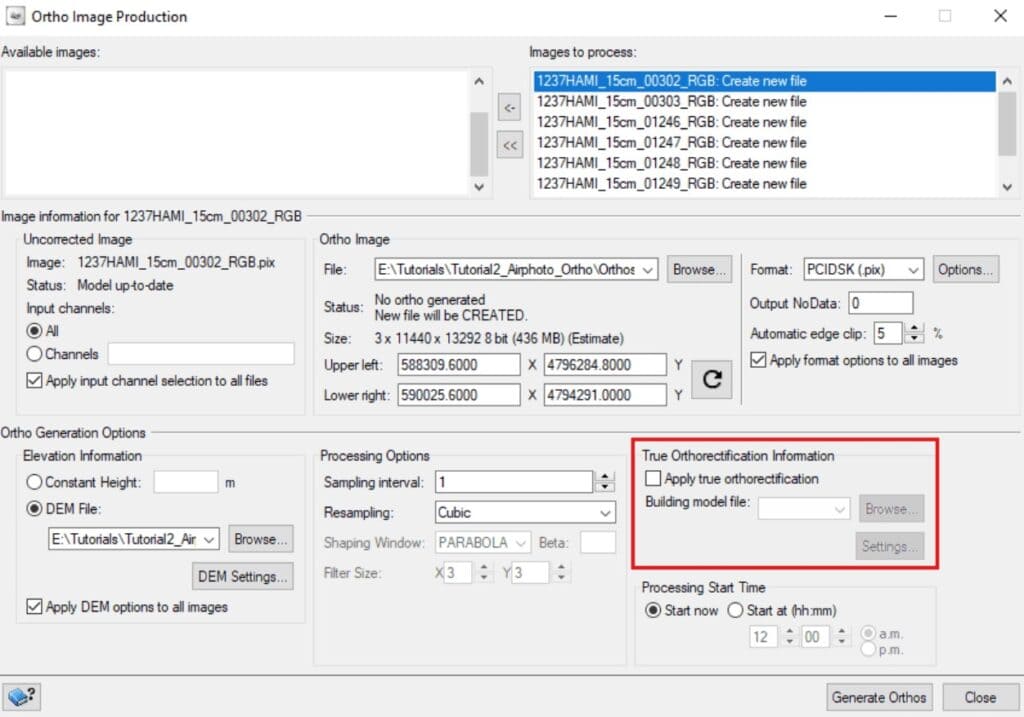
10.1 True Orthorectification
True orthorectification is an advanced form of orthorectification that corrects surface vertical structures, such as buildings, so they stand at their true-ground upright position, as if from a bird's-eye view.
Note: To run this operation, a building model for the selected area of interest is required.
To perform true orthorectification:
- In the Ortho Image Production window > True Orthorectification Information section, click the Apply true orthorectification checkbox.
- In the Building model file field, type in or select Browse to navigate to the path of your building model file. The Settings window opens.
- In the Settings window, specify the settings for each layer. You can learn more about this window on our Help webpage - Setting True-Orthorectification Options.
- Click Generate Orthos.
- Close the window and save the project.
For more information on orthorectification and true orthorectification, see our Orthorectifying Images and True Orthorectification and TORTHO documentation on our Help webpage.
11. Mosaicking
See the Mosaic Tool tutorial for a detailed guide on mosaicking in CATALYST Professional.
To mosaic the orthorectified images:
- In the same OE project, go to Processing step > Mosaic > choose Mosaicking.
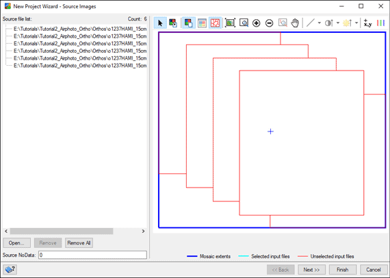
- The Mosaic Tool opens.
- The New Project Wizard – Source Images opens and loads the OE project imagery.
- Click Next.
- On the New Project Wizard – Mosaic Definition window, navigate to an output file location. Choose Pixel Size.
- Click Next.
- On the New Project Wizard – Mosaic Preparation window, modify the cutline and colour balancing methods to best suit your imagery.
- Click Generate Preview.
- Click Generate Mosaic.
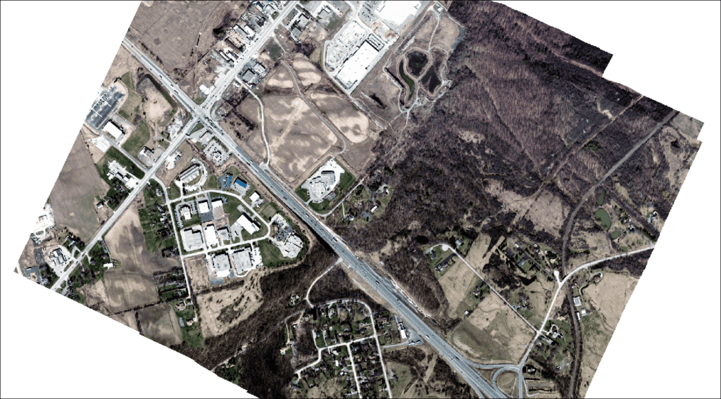
- This generates the output mosaic file, mos.pix.
- To view your mosaic, load mos.pix into Focus: