Building a Composite Mosaic

This tutorial demonstrates how to use the COMPOSITE algorithm within a workflow to download data from Microsoft’s Planetary Computer, ingest and merge into PCIDSK format, and generate a composite mosaic that selects the best pixels from each image.

The COMPOSITE algorithm applies a variety of pixel-based compositing techniques to merge geocoded images into a single mosaic. This process reduces noise, enhances useful information, and is particularly effective for removing clouds. The algorithm works with Analysis Ready Data (ARD) that includes either bitmap cloud masks or a quality/class layer identifying cloud pixels.

Note: All input imagery must share the same resolution and projection.

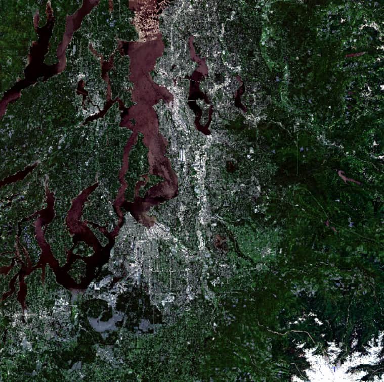
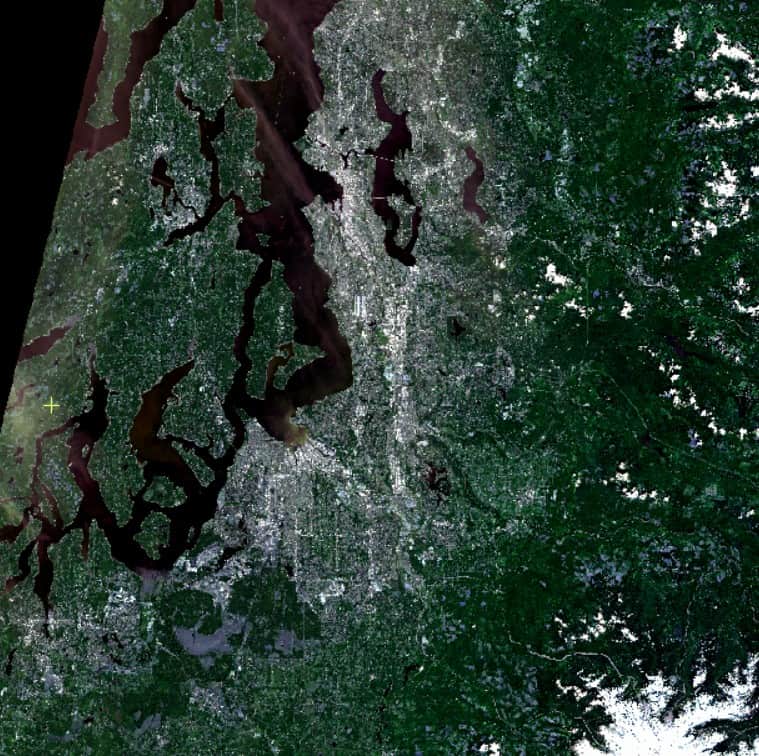
In this tutorial, we’ll demonstrate cloud-pixel removal by compositing three Sentinel-2 L2A images in Redmond, Washington.

Compositing Methods

The COMPOSITE algorithm mosaics images by applying rules to select each pixel. Six pixel selection techniques can be applied depending on the use case:

1. Median - selects the geometric median.
   • The median pixel is obtained from the image bands across the dates.
2. Medoid - selects the geometric mediod.
   • The medoid pixel is obtained from the image on the day whose set of bands is closest to the middle.
3. NDVI - chooses the pixel with the highest NDVI value.
   • Produces a mosaic with the most vegetation.
   • The opposite of the MinNDVI method.
   • Requires Red and NIR channels.
4. MinNDVI - chooses the pixel with the smallest NDVI value.
   • Produces a mosaic with the least vegetation.
   • The opposite of the NDVI method.
   • Requires Red and NIR channels.
5. Average - averages each pixel across the images and uses that in the output mosaic.
6. Date - chooses the pixel with the most recent date.

Masks & Classification Layers

Each input ARD file contains a classification or bitmap layer, which is used to identify cloud pixels. In Sentinel-2 L2A products, this channel is called the Scene Classification Layer (SCL). It groups pixels according to the table below:

COMPOSITE Workflow

Data Acquisition

ARD imagery can be obtained from various data providers. Microsoft's Planetary Computer is one of such providers that hosts various open datasets through a SpatioTemporal Asset Catalogue (STAC). This makes the data accessible through APIs and Python libraries. Although this cloud-based platform works with or without an API key, having one gives more permissive access to the data.

You can find helpful sample scripts and notebooks through their Quickstart webpage and GitHub repository

from pystac.extensions.eo import EOExtension as eo
import pystac_client
import planetary_computer
import os
import rioxarray

# Set the environment variable PC_SDK_SUBSCRIPTION_KEY, or set it here.
# The Hub sets PC_SDK_SUBSCRIPTION_KEY automatically.
## pc.settings.set_subscription_key(<YOUR API Key>)

# Using the pystac-client to search the STAC API for data subsets
catalog = pystac_client.Client.open(
    "https://planetarycomputer.microsoft.com/api/stac/v1",
    modifier=planetary_computer.sign_inplace,
)

# Get your AOI - near Redmond, Washington.
area_of_interest = {
    "type": "Polygon",
    "coordinates": [
        [
            [-122.27508544921875, 47.54687159892238],
            [-121.96128845214844, 47.54687159892238],
            [-121.96128845214844, 47.745787772920934],
            [-122.27508544921875, 47.745787772920934],
            [-122.27508544921875, 47.54687159892238],
        ]
    ],
}

# Specify your time range to filter images with
time_of_interest = "2019-06-01/2019-07-01"


# Apply your AOI and TOI in the catalog search
search = catalog.search(
    collections=["sentinel-2-l2a"],
    intersects=area_of_interest,
    datetime=time_of_interest,
    query={"eo:cloud_cover": {"lt": 25}},
)

items = search.item_collection()

Data Ingest

The search result produces 'items' corresponding to a scene in the collection. Each scene has assets that provide the bands as Cloud Optimized GeoTIFFs (COGs) and metadata as XML files through downloadable links. Since the bands are available individually, they can be downloaded using the Rasterio and Rioxarray Python packages and compiled into a multichannel PCIDSK file using the DATAMERGE algorithm.

outdir = os.getcwd()
for item in items:
    outdir = os.path.join(os.getcwd(), item.id)
    assets = item.assets

    if not os.path.exists(outdir):
         os.makedirs(outdir)
    else:
        continue

    for band, asset in assets.items():

        # Selecting the RGB, NIR (10 m) and SCL bands
        if band in ['B02', 'B03', 'B04', 'B08', 'SCL']:
            link = asset.href
            title = asset.title

            # Creating raster array
            tif_file = rioxarray.open_rasterio(link, default_name=title)
            outfile = os.path.join(outdir, band + ".tif")

            # Downloading bands as COGs
            tif_file.rio.to_raster(outfile,
                                   driver="COG",
                                   dtype="uint16",      # Sentinel-2 bands are 16-bit
                                   compress="deflate",
                                   overwrite=True)
    

    # Merging tiff bands into multichannel pix file using DATAMERGE
    from pci.datamerge import datamerge
    mfile = outdir
    filo = os.path.join(outdir, item.id + ".pix")
    dbic  = []
    ftype = ""
    foptions = ""
    extent = "UNION"
    nodatval= []
    resample=""

    datamerge(mfile, dbic, filo, ftype, foptions, extent,nodatval,resample)

    # Write path to each pix image into comp_mfile => list of all merged files => pix files of all scenes
    comp_mfile = os.path.join(os.getcwd(), "composite_mfile.txt")
    with open(comp_mfile, "a") as file:
        file.write(f'"{filo}"' + "\n")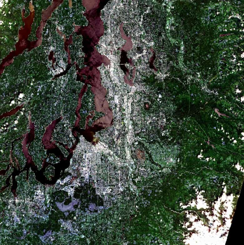

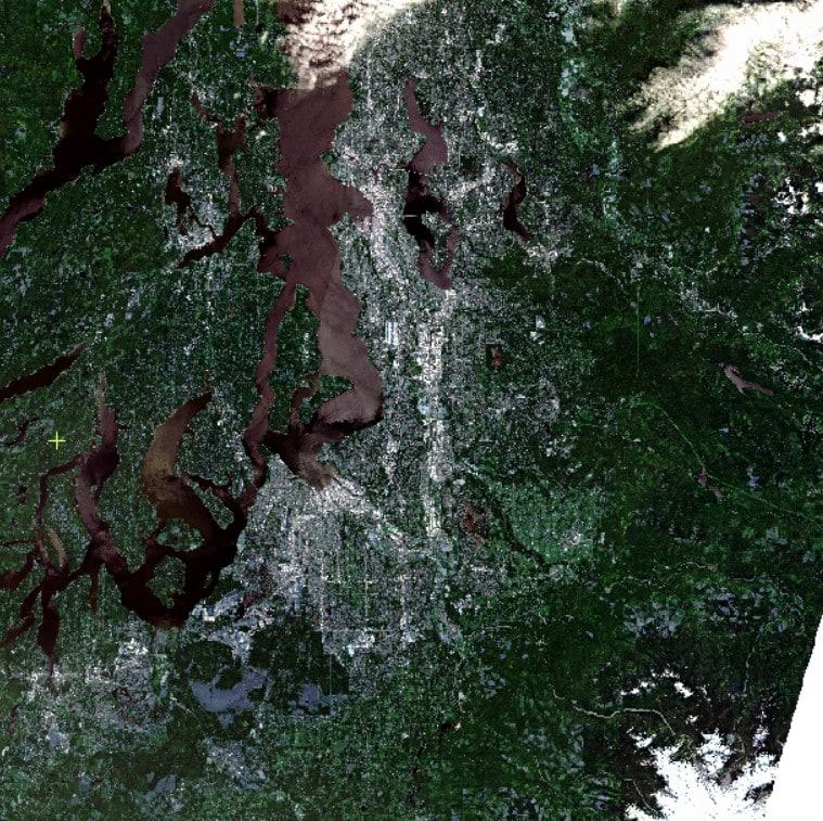
Running COMPOSITE

The following Python script mosaics the three Sentinel-2 L2A scenes into a single image to remove cloud cover. It uses the SCL channel with values 3, 8, 9, and 10 corresponding to cloud shadows, medium and high cloud probability and thin cirrus, respectively, to indicate the cloud pixels to exclude. The fill option also makes sure that in worst-case scenarios where no good pixels are found, it uses an excluded value rather than having 'holes' in the image.

from pci.composite import composite
import os

##  MEDIAN COMPOSITE
mfile    = r"<path to mfile>"     # List of geocoded image files
dbimage  = [1, 2, 3, 4]           # List of image bands to be in mosaic
mfilemsk = ""
dbicmask = [5]                    # input channel containing the class information
maskvals = [3, 8, 9, 10]          # list of exclusion values in DBICMASK channel
dbib     = []
filo     = os.path.join(os.getcwd(), "RGB_median_mosaic_nofill.pix")
compmeth = "MEDIAN"               # compositing method
dbicndvi = []
dateto   = []
datefrom = []
dayspan  = []
compopts = "fill smooth"          # compositng options

composite(mfile, dbimage, mfilemsk, dbicmask, maskvals, dbib, filo, compmeth,
          dbicndvi, dateto, datefrom, dayspan, compopts)

Result

The resulting image merged the input files using the median method and cloud exclusion values from the SCL channel to produce an image with reduced cloud cover.