Optical Satellite Orthorectification

Orthorectified images (orthos) are geometrically corrected and georeferenced imagery. Orthorectification is the process of using a rigorous math model and a digital elevation model (DEM) to correct distortions in raw images.

This tutorial outlines the optical satellite orthorectification process using OrthoEngine. This workflow will show how to import data, collect ground control points (GCPs) and tie points (TPs), and then orthorectify the images. Kompsat-3 data of Toronto, ON will be used for this tutorial, however these same steps can be followed with other types of optical satellite data. 

More information on each of the steps that are run in this tutorial is included in the online Help Documentation for CATALYST Professional.

PROJECT SETUP AND DATA INGEST

Follow the steps below to create an OrthoEngine project, choose the appropriate math model, and add your imagery.

SETTING UP THE ORTHOENGINE PROJECT

To create a new OrthoEngine project:

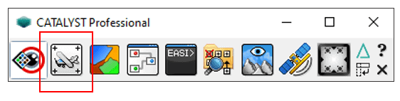
1. Open OrthoEngine from the CATALYST Professional toolbar
   
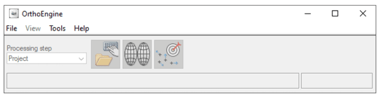
2. The OrthoEngine toolbar opens. Navigate to File > New.
   
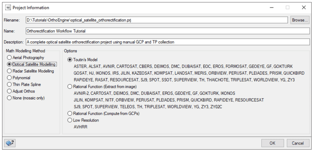
3. The Project Information window opens.
   • Give your project a Filename, Name and Description.
   • Under Math Modeling Method, select Optical Satellite Modelling.
   • Under Options, select appropriate model. For this tutorial, we will choose Toutin’s Model.

OPTIONS FOR MODELLING

Toutin’s Model – A rigorous model that compensates for known distortions to calculate position and orientation of the sensor at time of image acquisition. Suitable for use with any optical satellite data, regardless of resolution, such as CARTOSAT, LANDSAT, or SPOT.

Rational Function (Extract from image) and Rational Function (Compute from GCPs) – Simple math models that builds correlations between pixels and ground locations. They can be applied to any image dataset. Use this math model in the following situations:

• The sensor model is proprietary (classified).
• The image has been processed geometrically.
• The data provider computed the math model and distributed it with the image.
• You do not have the whole image.
• Information needed for a rigorous math model, e.g., the orbital segment containing the viewing geometry which generates the rational polynomial coefficients (RPCs), is missing.
  • To import the RPCs from a file, select Rational Function (Extract from image).
  • When the RPCs are calculated based on the GCPs that you collect, select Rational Function (Compute from GCPs).

 Low Resolution – For use with advanced very-high-resolution radiometer (AVHRR) data.

For more information on choosing a math model, click on the CATALYST Help button or search Creating a project and selecting a math model in the CATALYST Help.

4. Click OK.

Note: At this point, it’s a good idea to save the project via File > Save. This saves your orthorectification progress to the OrthoEngine project (.PRJ) file.

PANSHARPENING THE IMAGERY (OPTIONAL)

If you wish to pansharpen your imagery, you can do so at this point.

With many data products, such as Worldview/Quickbird Ortho-Ready Standard data, SPOT, and Pleiades, the PAN and MS images are resampled exactly on top of each other. Therefore, it is possible to perform pansharpening of the data before orthorectification.

To pansharpen the images:

• From the OrthoEngine toolbar > Tools > Merge/Pansharp Multispectral Image. Once the data is pansharpened, it will be added to the OrthoEngine project.

ADDING THE IMAGERY

Check the CATALYST Sensor Support page to see if your sensor data is supported.

Note: Search the sensor name of your imagery in CATALYST Help to determine which key file type to use to open the image. For example, the key file name for KOMPSAT-3 is *_aux.xml.

To add imagery:

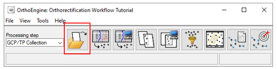
1. On the OrthoEngine toolbar > Processing Step > Choose GCP/TP Collection.
2. Click the Open a new or existing image button.
   
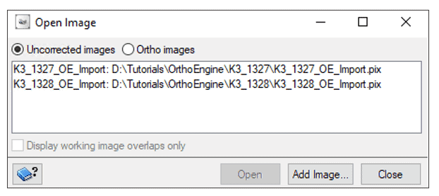
3. The Open Image window opens. Click Add Image.
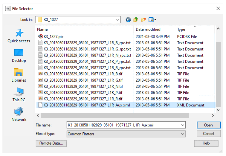
4. From the File Selector window, navigate to the folder containing your first image file.
   • For the tutorial dataset we open the folder for image K3_1327.
5. Select the sensor’s key file from the folder.
   • For KOMPSAT-3 data, select the *_aux.xml file: K3_20130501182829_05101_19871327_L1R_Aux.xml
     
6. Click Open.
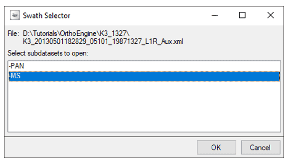
7. The Swath Selector window opens. Choose the MS bands subdataset, click OK.
   
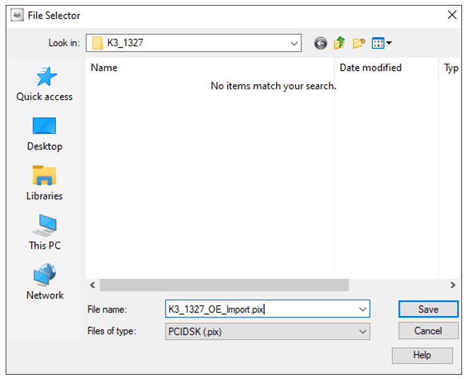
8. A question window appears, reading Do you want to import data file to PIX file to optimize processing? Click Yes.
9. A File Selector window opens. Type a File name for the PIX file output.
   
10. Click Save.
11. A question window appears, reading Do you wish to create overviews now? Click Yes.
12. Your new PIX file now appears in the Open Image window.
13. Repeat Steps 3-11 for your second image. The Open Image window now lists both uncorrected images.
    
14. Click Close.

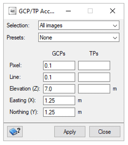
SET GCP/TP ACCURACY

Prior to collecting ground control points (GCPs) and tie points (TPs), you’ll want to verify and adjust the GCP/TP Accuracy settings for your project. Setting the proper accuracy values is very important. For example, if your project consists of surveyed GCPs, the accuracy entered should be <1.0 metre.

For more details on setting the accuracy of GCPs and TPs, search Setting the accuracy values in CATALYST Help.

To set GCP/TP accuracy:

1. On the OrthoEngine toolbar > Processing Step > Choose GCP/TP Collection.
2. Click the GCP/TP Accuracy button.
   
3. The GCP/TP Accuracy window opens.
   • From Selection, choose the images of which you wish to adjust the accuracy.
     • For this tutorial, we select All images.
   • From Presets, you can choose preset accuracy parameters grouped as: Default values, Surveyed GCPs, High-accuracy GCPs, Medium-accuracy GCPs, or Low-accuracy GCPs.
     • For this tutorial, we select None.
   • Under GCPs, TPs, or both, manually enter the parameters by which to set the accuracy of points in the image coordinate system, Pixel and Line, and the ground coordinate system, Elevation (Z), Easting (X), and Northing (Y), as applicable.
     • For this tutorial, we manually chose GCP accuracy in the medium- to high-accuracy range.
       
4. Click Apply. Close GCP/TP Accuracy window.

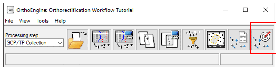
COLLECT GCPS

Now that the images are imported and the accuracy is set, you can collect GCPs in order to improve absolute accuracy in the model.

AUTOMATICALLY COLLECTING GCPS

For details on choosing the optimal number of GCPs and TPs for your project, search Collecting the right number of ground control points in CATALYST Help.

To collect GCPs automatically:

1. On the OrthoEngine toolbar > Processing Step > Choose GCP/TP Collection.
2. Click the Collect GCPs Automatically button.
   
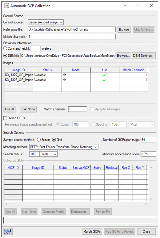
3. The Automatic GCP Collection window opens:
   • For Control source, choose Georeferenced Image.
   • For Reference file, browse to your desired reference image. For this tutorial, we will use the SPOT o2_5m.pix file.
     

CHOOSING A REFERENCE IMAGE AND OPTIMAL SEARCH OPTIONS

For details on choosing the appropriate reference image, search Using geocoded or raw images for collecting ground control points in CATALYST Help.

For more details on the Search Options, search Collecting ground control points automatically in CATALYST Help.

• Under Elevation Information, choose DEM file and browse to your desired DEM file. For this tutorial, we will use the dem_30m.pix file.
• If required, adjust Search Options.
  • For this tutorial, we’re leaving the Search Options with the default parameters.
    

4. Click Match GCPs.

Once the procedure is complete, the collected GCPs will be listed under the Collected GCPs section.

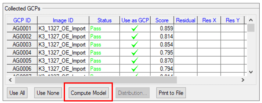
COMPUTING THE MODEL

OrthoEngine calculates a temporary model using any existing data in the project file plus the newly collected GCPs, but the model is not saved in the project file. In the Collected GCPs table, you can scroll to the right to view additional columns, including residual errors.

To compute the model:

1. Click Compute Model to view the residuals for each of the GCPs.
   
2. Now the residuals are visible in the table. Click on Residual to sort the GCPs from highest to lowest residual.
   
3. If you are satisfied with the GCPs in the list, click Add GCPs to Project. Skip ahead to Step 4.
4. If you want to adjust the GCPs collected, read Step 3.3.

Note: You can choose to run the Automatic GCP collection again after adding the points to the project.

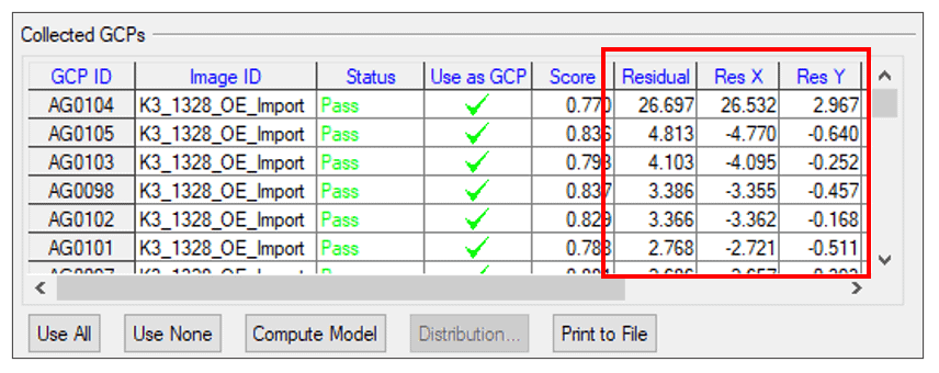
REFINEMENT (OPTIONAL)

At this point, you can choose to refine the GCP collection parameters, if desired.

To refine the GCPs:

1. Change the Search Options and recollect GCPs by clicking Match GCPs again.
2. Additionally, you can select which GCPs to use from the list of collected GCPs. If some GCPs have too high a residual, you have the option to remove them from calculations.

To remove a GCP from the model calculations:

1. Click on the checkmark in the Use as GCP column to unselect it.
2. Click Compute Model again.
   
3. Once you are satisfied with the GCPs in the list, click Add GCPs to Project.
4. Close the GCP Collection window.

Note: You can also choose to rerun the GCP collection after adding to the project.

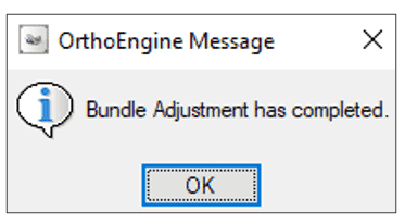
CALCULATING THE MATH MODEL

OrthoEngine recalculates the math model several times to find the best possible solution. That is, when residual errors of the GCPs and TPs occur within the limit set in the thresholds of the x, y, and z coordinates or the angles, or until the limit in number of iterations is reached.

To calculate the math model:

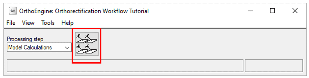
1. On the OrthoEngine toolbar > Processing Step > Choose Model Calculations.
2. Click the Compute Model button.
   
3. A bundle adjustment is executed on the data.
   

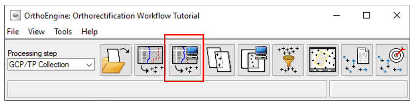
COLLECT TPS

Since we have two images and want to ensure that the two images match each other, we will collect tie points (TPs) in order to further improve relative accuracy in the model. To automatically collect TPs:

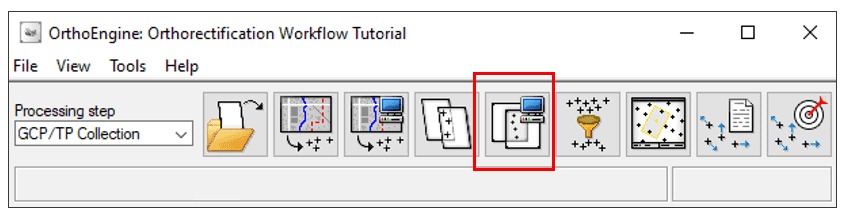
1. On the OrthoEngine toolbar > Processing Step > Choose GCP/TP Collection.
2. Click the Automatically collect tie points button.
   
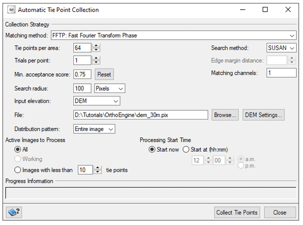
3. The Automatic Tie Point Collection window opens. Under Collection Strategy:
   • For Matching method, choose FFTP: Fast Fourier Transform Phase from the dropdown.
   • For Input elevation, choose DEM from the dropdown. Browse to and select your DEM file.
   • The DEM window appears. Leave as default parameters and click OK.
   • If required for your dataset, adjust the other parameters.
     
     Note: For more details on parameters for collecting TPs automatically, click on the CATALYST Help button or search Understanding automatic tie-point collection in CATALYST Help.
     
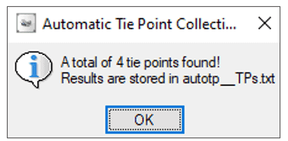
4. Click Collect Tie Points.
5. A pop up will appear to tell you how many TPs were collected. The number of TPs collected will be based on factors such as amount of overlap available between images. Click OK.
   
6. Under Progress Information, it reads Tie point collection complete.
7. If you want more or fewer TPs than what was collected, you can now adjust the parameter values and run the process again.
8. Close the Automatic Tie Point Collection window.
   

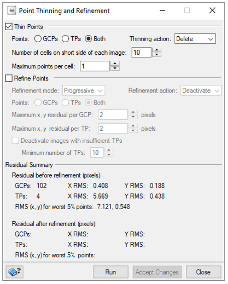
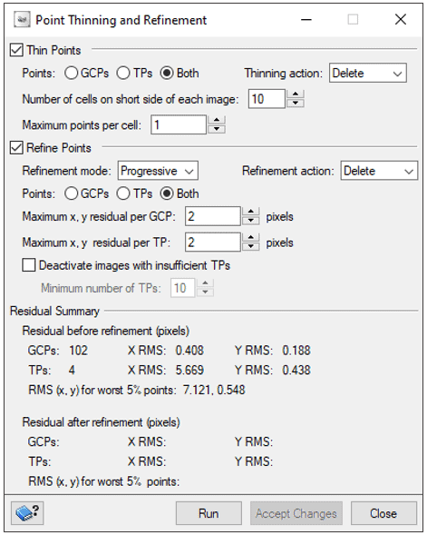
POINT THINNING AND REFINEMENT

After you have collected GCPs and TPs, you can choose to further refine them.

If necessary, you can thin points to remove those that are redundant. You can also refine points that have a high root mean square (RMS). That is, you can opt to run thinning, refinement, or both simultaneously. When you select to have thinning and refinement run simultaneously, thinning occurs first with refinement immediately thereafter.

Typically, you run thinning, refinement, or both, after you have run automatic point collection and, as a result, have redundant points in an over-collected region or points that have a high RMS due to poor correlation.

Note: Make sure to calculate the model (Processing Step > Model Calculations > Compute Model) before this step.

To open the thinning and refinement options:

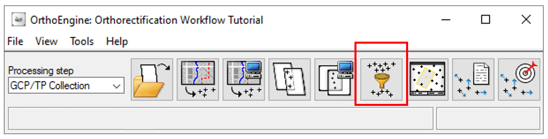
1. On the OrthoEngine toolbar > Processing Step > Choose GCP/TP Collection.
2. Click the Point Thinning and Refinement button.
   
3. The Point Thinning and Refinement window opens.

POINT THINNING

To set up point thinning, select the type of points you want to thin, how you want to dispose of the points designated for removal, and then define the grid by which to divide the image into cells. By defining the grid, you can specify how many points you want to retain in each cell.

To set up point thinning:

1. Check off the Thin Points box.
   • Points – Select the type of points you want to thin: GCPs, TPs, or Both.
   • Number of cells on short side of each image – Enter the number of cells on the short side of each image. For example, with an image that has an aspect ratio of two to one (2:1), and you want to indicate that the short side has 10 cells (and, therefore, the long side has 20 cells), enter 10. That is, the image has 200 cells.
   • Maximum points per cell – Enter the number of points to retain in each cell.
   • Choose a Thinning action:
     i. Deactivate – Designate removed points as inactive but does not delete the point. You can switch deactivated points back to active in the future.
     ii. Delete – Permanently remove the points from the project.
2. For the tutorial, we will leave the settings as the default values. If you are satisfied with point-thinning only, uncheck Refine Points and click Run.
   

If you also want to refine the points, continue to the next section.

POINT REFINEMENT

To set up point refinement, select the type of points you want to refine, the mode to use, how you want to dispose of the points designated for removal, and then enter the maximum x and y residual per point.

To set up point refinement:

1. Ensure the Refine Points box is checked.
   • Choose a Refinement Mode:
     i. Progressive – Reject points iteratively. Points with a very high RMS threshold will be removed. The threshold is reduced iteratively based on the maximum x and y residual you specify.
     ii. Direct – Reject points at a specific threshold. Points are rejected at precisely the maximum x and y residual you specify.
   • Points – Select the type of points you want to thin: GCPs, TPs, or Both.
   • Maximum x, y residual per GCP/TP – Enter a value into either or both boxes depending on your points choice. This value represents the threshold at which to reject the relevant points.
   • Deactivate images with insufficient TPs – Deactivates images that do not have enough TPs. You would then specify the threshold in the Maximum number of TPs box.
   • Choose a Refinement action:
     i. Deactivate – Designate removed points as inactive but does not delete the point. You can switch deactivated points back to active in the future.
     ii. Delete – Permanently remove the points from the project.
     
2. For the tutorial, we will leave the settings as the default values. Once you are satisfied with the thinning and refinement configuration, click Run.
   • You can also choose to only refine points. In that case, uncheck Thin Points.

Tip: If necessary, you can rerun the process with different settings, and compare the residual summary of each.

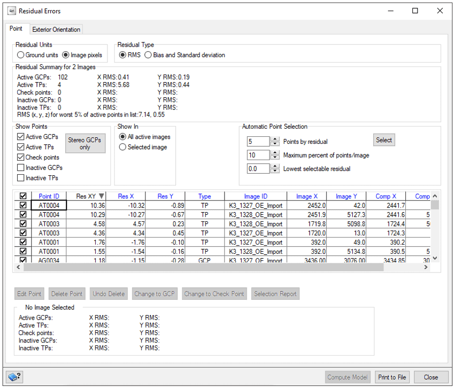
RESIDUAL REPORT

A residual report helps you determine if the math-model solution is of sufficient quality for your project. The residual errors the report contains do not necessarily reflect errors in the GCPs or TPs, but rather the overall quality of the math model.

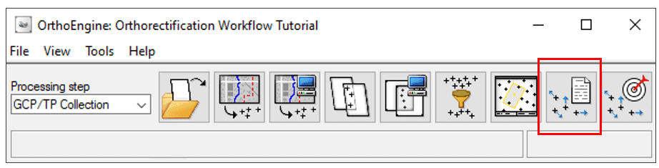
To view the residual report:

1. On the OrthoEngine toolbar > Processing Step > Choose GCP/TP Collection.
2. Click the Residual report button.
   
3. The Residual Errors window opens. The collected GCPs and TPs are displayed in this window.
   Note: For explanations of each of the options, search Generating a residual report for points in CATALYST Help.
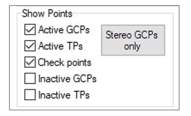
4. Under Show Points, you can choose to look at Active GCPs, Active TPs, Check points, Inactive GCPs, or Inactive TPs. 
   
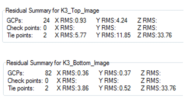
   When you click on one of the points in the table you can see the residual summary for each image.
   
5. If you have any points with very high residual errors, you can remove them from the model using the Delete Point button.
6. Once you are satisfied click Compute Model and then Close the window.
   

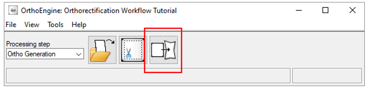
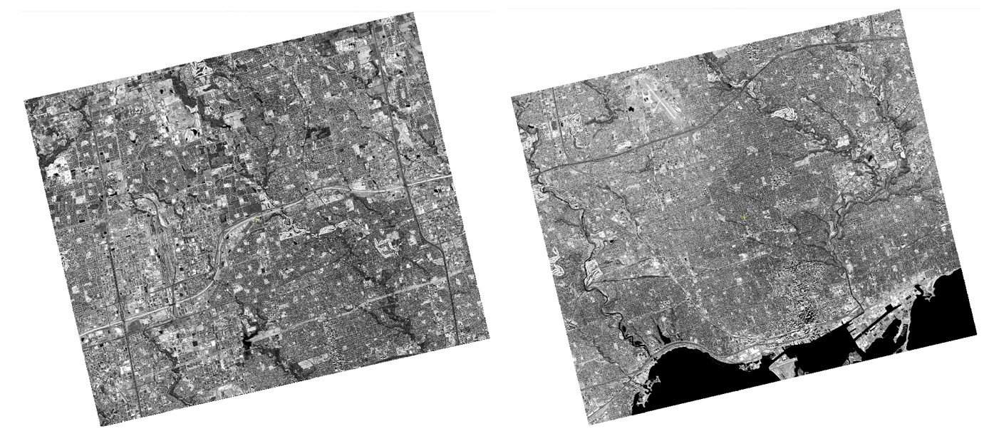
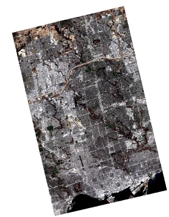
GENERATE ORTHO IMAGES

You can now generate the orthorectified images – geometrically corrected and georeferenced.

To generate orthorectified images:

1. On the OrthoEngine toolbar > Processing Step > Choose Ortho Generation.
2. Click the Schedule Ortho Generation button.
   
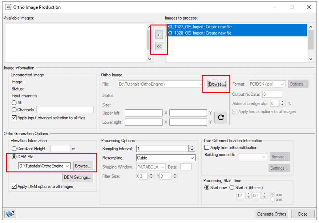
3. The Ortho Image Production window opens.
   • Select the images in the left panel and add them to the right panel.
   • Browse to the output location for your ortho images.
   • Select the DEM.
     
4. Click Generate Orthos.
5. Once the ortho step is complete, you will have two orthorectified images. They are saved as PIX files with the naming convention of o*_.pix, where * is the name of the PIX file of the raw image.
   

• Select the DEM.
  

Tip: Please also refer to our in-depth mosaicking tutorials for more information: Automatic Mosaicking and Manual Mosaicking.