Object Analyst Classification

Object Analyst is an object-based image-analysis (OBIA) module. It is used to segment an image into objects for classification and analysis. It differs from the traditional pixel-based approach, which focuses on a single pixel as the source of classification.

Object Analyst is for use primarily with very-high-resolution (VHR) imagery. The tool can be used with any imagery, however, that meets the necessary criteria. That is, you can use imagery of lower resolution, of various resolutions, and of any input format supported by CATALYST Professional.

Object Analyst in CATALYST Professional provides an intuitive workflow wizard for performing image segmentation, classification, and feature extraction. This all-in-one interface is designed to reduce complexity and give users the opportunity to develop highly accurate, object-based, thematic classification maps.

More information on each of the steps that are run in this tutorial is included in the online Help Documentation for CATALYST Professional.

THE TUTORIAL DATA

Download the tutorial data package. The data package should include the following file:

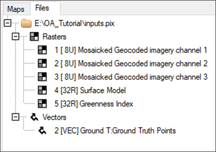
inputs.pix – A PCIDSK file (.PIX) is a proprietary file format of CATALYST Professional which can contain many raster channels, vector layers, and other auxiliary information. This file contains:

• 3 imagery channels (RGB),
• 1 surface model,
• 1 greenness index channel, and
• 1 vector layer containing ground truth points.

Note: The surface model and greenness index channels can be generated using algorithms and tools available in CATALYST Professional.

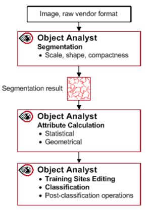
OBJECT ANALYST WORKFLOW

The CATALYST Professional Object Analyst workflow includes the following steps:

1. Segmentation
2. Attribute calculation
3. Training sites editing
4. Supervised classification
5. Unsupervised classification
6. Rule-based classification
7. Post classification editing
8. Accuracy assessment

The Object Analyst flowchart below outlines the inputs, order of operations, and intermediary results. 

DATA PREPARATION

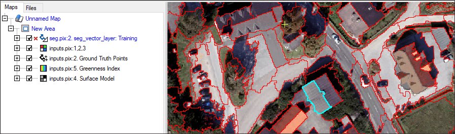
Before opening the Object Analyst wizard, load your data file and examine the different layers that will be used as inputs to the segmentation and object-based classification.

To load and examine your input file:

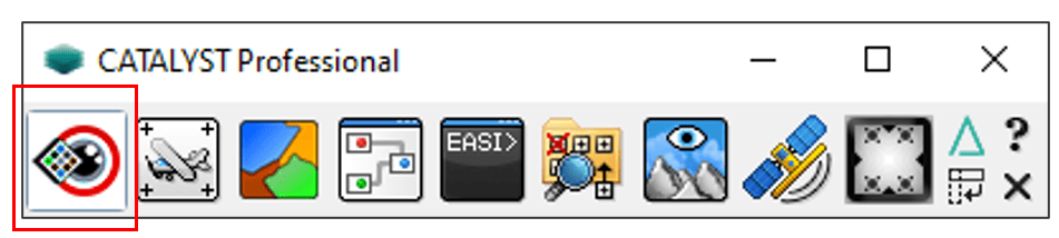
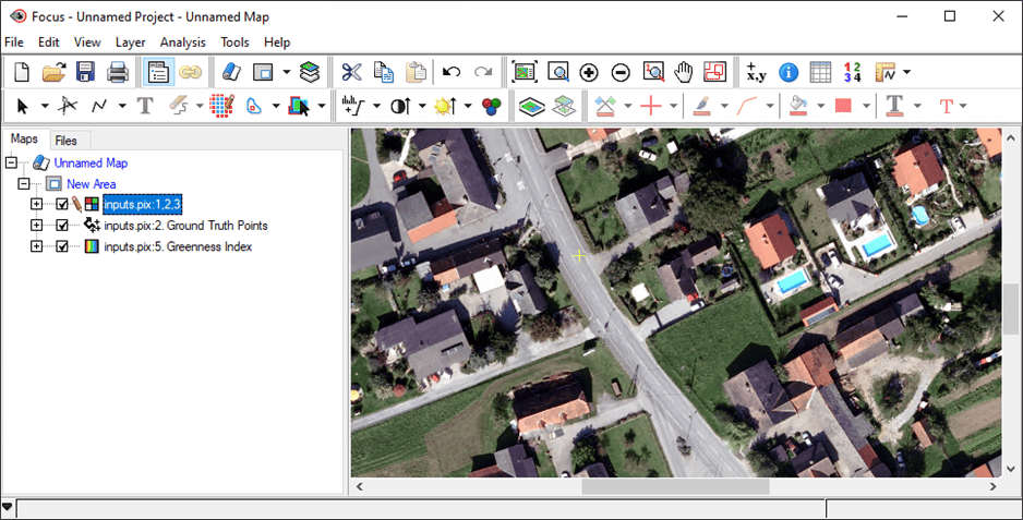
1. Open Focus from the CATALYST Professional toolbar.
   
2. Go to File > Open.
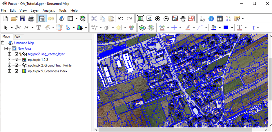
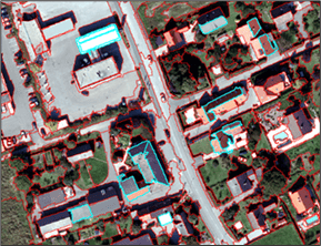
3. Navigate to the folder that you downloaded inputs.pix to and click Open. The image will automatically load as a true color composite (R:1, G:2, B:3).
   
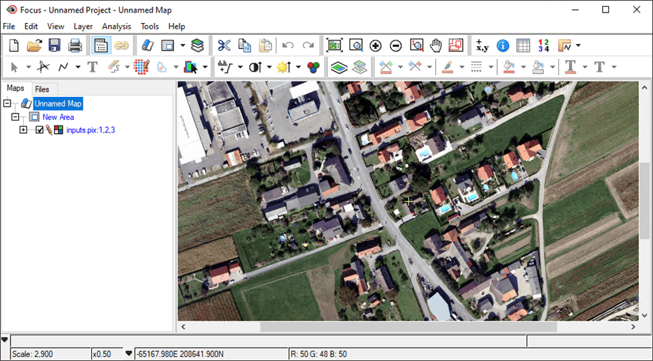
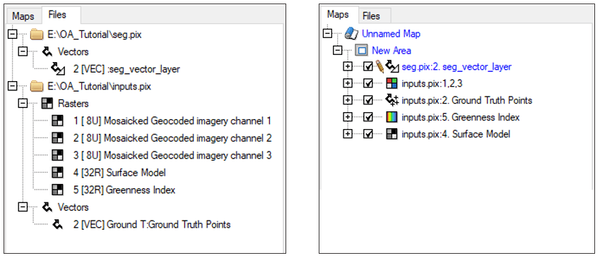
4. Click on the Files tab. Expand the Rasters and Vectors branches to view the individual layers contained in the PIX file.
   
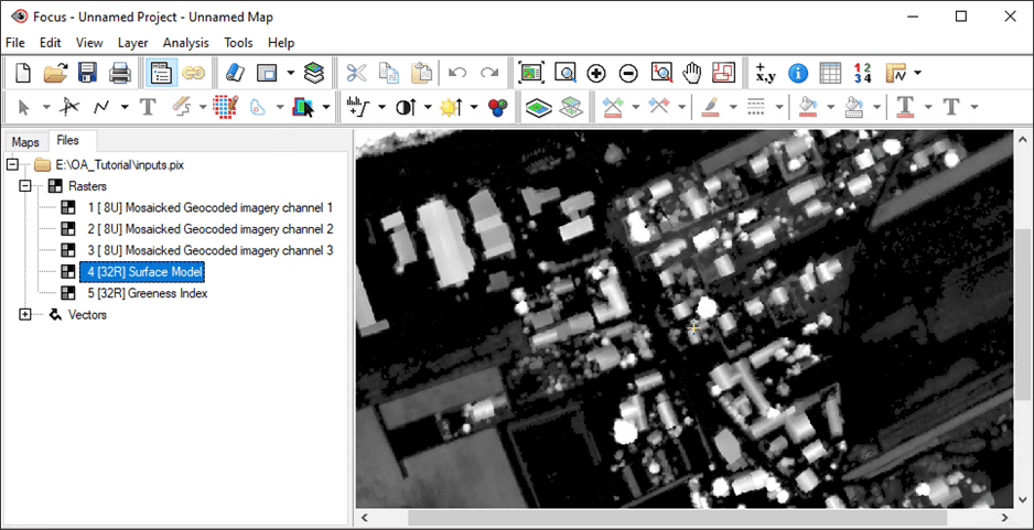
5. Right click on the Surface Model layer and select View > As Grayscale. A normalized Surface Model will render in grayscale.
   
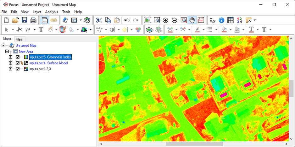
6. Right click on the Greenness Index and select View > As Pseudocolor. To adjust the pseudocolor representation:
   • Under the Maps tab, right-click the Greenness Index layer, select Edit PCT. The PCT Editing window opens.
   • Under the Single Value tab, from the Predefined Pseudocolor Tables, choose Smooth. Click Close.
   • The rendering now clearly represents areas that are relatively more green. Areas in red represent high amounts of green color, whereas areas in green represent lower amounts of green color.
     
7. The final layer in the inputs.pix file is the Ground Truth Points vector file. Right click the segment and click View. The points will then be loaded.
   • This segment will be used in the section Training Sites Editing – Importing Ground-Truth Points.
8. Switch to the Maps tab and uncheck the other layers to view your vector points.
   
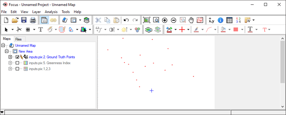
9. Move the RGB layer to the top so that the true color composite is rendering in the viewer.
   

Note: Saving the project frequently will help optimize processing speeds throughout the Object Analyst workflow.

SEGMENTATION

The first task in performing object-based classification is to divide a scene into homogeneous regions, or segments. Performing segmentation consists of selecting one or more source-image layers (e.g. feature heights layer, greenness index layer, etc.) and choosing segmentation parameters, which consists of values for scale, shape, and compactness.

To set up and perform segmentation:

1. In Focus, click Analysis > Object Analyst. The Object Analyst wizard opens.
   
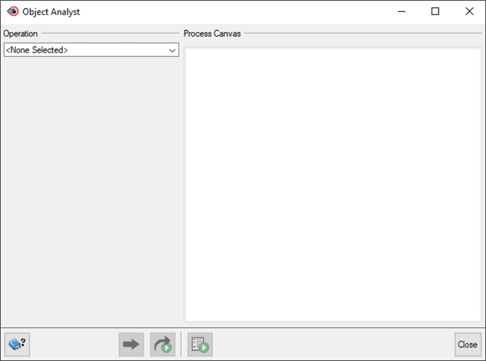
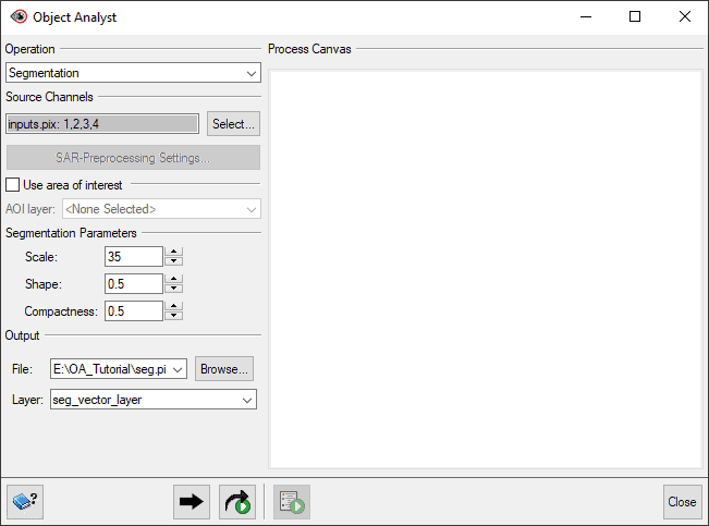
2. From the Operation dropdown list, select Segmentation.
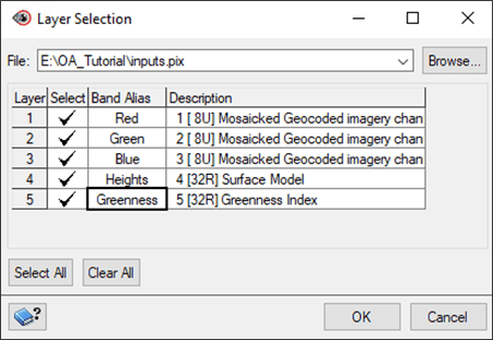
3. In the Source Channels section, click Select. The Layer Selection window opens:
   1. In the File dropdown list, select the inputs.pix file.
   2. Under the Select column, check the first 4 channels (not the 5th). The layers selected in this panel will be used as input for segmenting the image.
      
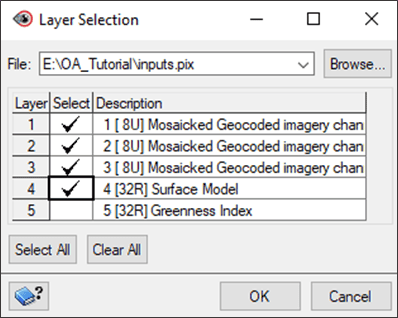
   3. Click OK.
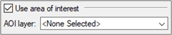
4. For this tutorial, leave the Use area of interest unchecked.

SETTING AN AREA OF INTEREST

To help keep processing time down, there is the option to set an area of interest (AOI). This is especially useful for larger projects. The segmentation will then be constrained to a specified area.

To set an AOI:

1. In Focus, open the .PIX file (and layer) containing the polygons that you want to use so that they will be available in the Object Analyst wizard.
2. From the Object Analyst window, select the Use area of interest check box.
3. For AOI layer, click the dropdown and select the available vector layer containing the polygons you want.

For more information on different AOI scenarios, click on the CATALYST Help button or search Constraining segmentation to an area of interest in the CATALYST Help.

5. In the Segmentation Parameters section, set Scale to 35.

Note: Some experimentation with values for the Segmentation Parameters may be necessary to achieve the result you want. A lower shape value (e.g. 0.1) places high emphasis on color, which is typically the most important aspect of creating meaningful objects. A higher compactness weighting (e.g. 0.9) can produce object boundaries that are more compact, such as with crop fields or buildings.

6. In the Output section, name the output file and layer:
   • For File, click Browse. In the File Selector window, type seg.pix and click Save.
   • For Layer, click the field and type the name of the new vector layer on which the segmentation results will be saved, seg_vector_layer.
     
7. Click the Add and Run button .
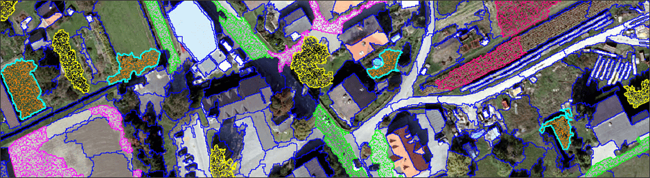
8. After processing has completed, the segmentation layer will appear on the Process Canvas, and the results are loaded into the Focus view pane.
   
   

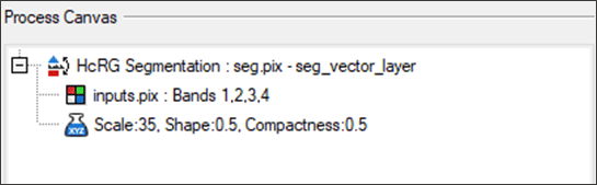
Note: Under the Files tab, you can see the name of the saved file, seg.pix, and by expanding the Vectors branch, you can see the name of the vector layer. Under the Maps tab, you also see the vector layer listed, seg_vector_layer, because it has been automatically loaded into the view pane.

ATTRIBUTE CALCULATION

With an attribute calculation, various attributes (e.g. geometrical, statistical, etc.) are computed for each polygon segment, or object.

Note: Each time you set up attribute calculation, Object Analyst uses, by default, the same raster channels and segmented vector file as specified for a previous segmentation operation.

To set up and run Attribute Calculation:

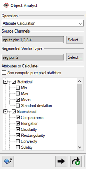
1. In the Object Analyst wizard, click on the Operation dropdown list and select Attribute Calculation.
2. In the Source Channels section, click Select. The Layer Selection window opens:
   1. Keep Channels 1 – 4 selected, but this time also check Channel 5 – Greenness Index.
   2. Change the Band Alias names to the following: B01 > Red, B02 > Green, B03 > Blue, B04 > Heights, B05 > Greenness.
      
3. Click OK.
4. In the Segmented Vector Layer section, the output from the segmentation step, seg.pix, will already be selected.
5. In the Attributes to Calculate section:
   • Expand the Statistical section and check Mean.
   • Expand the Geometrical section and check the following: Compactness, Elongation, Circularity, and Rectangularity.

Note: For more information on attributes to calculate, click on the CATALYST Help button or search Setting up and running Attribute Calculation in the CATALYST Help.

6. Click Add and Run .

Once the process completes, the outputs will be added to the Process Canvas.

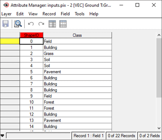
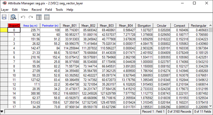
THE ATTRIBUTE MANAGER

The Attribute Manager is another way of visualizing and verifying the data. Each record in the Attribute Manager represents a shape on the layer, and each shape is described by a number of attributes.

To view the Attribution Manager:

1. In the Maps tab in Focus, right click on pix:2. seg_vector_layer and select Attributes Manager. The Attribute Manager table opens.
2. You should see a number of new columns with the headers that you just created in the previous step (e.g. Mean_red, Mean_green, Mean_blue, Rectangularity, etc).
3. Close the Attribute Manager window. 
4. Note: For more information on using the attribute manager, click on the CATALYST Help button or search Working with the Attribute Manager in the CATALYST Help.
   

TRAINING SITES COLLECTION

Before you can perform a classification or an accuracy assessment, you must have ground-truth data. With ground-truth data, image data can be related to real attributes and materials on the ground.

With supervised classification, the ground-truth data acts as a training set, which is used by the learning algorithm to generate a classification model. In Object Analyst, you collect training samples for both the supervised classification (called training sites) and accuracy assessment (called validation sites) in the same window.

To run Training Sites Collection:

1. In the Object Analyst wizard, change the Operation to Training Sites Editing.
2. Make sure that the Training Vector Layer is the layer you created in the Segmentation section of this tutorial, 2 [VEC]:seg_vector_layer.
3. There are two steps to the process of preparing training sites:
   1. Training sites: Manually selecting training sites by adding segmentation polygons to classes.
   2. Validation sites: Importing a point file that contains ground-truth information to verify the training class polygons.

SELECTING TRAINING SITES

Using on-screen interpretation in the viewer, users select segments of various classes to use as training polygons for the classification.

To manually collect training sites:

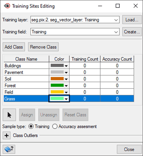
1. Under the Training Vector Layer section, click Edit. The Training Sites Editing window opens.
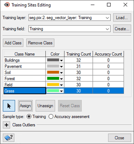
2. Ensure that Training Field is set to Training.
3. Click on Add Class. A new row is added that reads Class 1 under the Class Name column.
4. Change the name to the first class. For this tutorial, type Buildings.
5. Click on the Color dropdown to select a color to represent that class. For this tutorial, dark grey.
6. Repeat Steps 3-5 to identify the remaining classes, as shown below.
   
7. Highlight the Buildings class and then click on the Individual Select tool .
8. In the Focus viewer, select a segmentation polygon that overlaps a building.
   
9. Click the Assign button on the Training Sites Editing window, to add it to the Training Count column for your Buildings class.
   
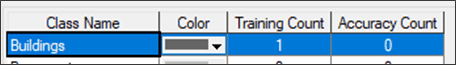
10. In the Focus viewer, hold the CTRL key down to select multiple polygons. Select at least 30 segmentation polygons that overlap buildings, making sure to select of different roof colors and styles.
    
11. Once you have selected a number of different building polygons, click Assign. The total count of polygons will appear under the Training Count column.
    • Once you have clicked Assign, click a random polygon to unselect all the polygons for this class.
      
      Note: You can save your .PRJ any time and the training site collection progress will be saved.
      
12. Highlight the next class in the table.
13. Repeat Steps 10-12 for the remaining four classes, making sure to collect at least 30 shapes for each. Try to be as accurate and diverse in your collection as possible.
    
14. Close the Training Sites Editing window.

Note: For your Accuracy Count, you have the option to either:

• repeat the steps above to manually collect validation sites, or
• Import Ground Truth Points as explained in the section below.

For more information, click on the CATALYST Help button or search Using the Training Sites Editing window in the CATALYST Help.

IMPORTING VALIDATION SITES

Ground-truth points, called validation sites, are used for the Accuracy assessment in Object Analyst.

To import a ground-truth vector layer:

1. From the Object Analyst wizard Training Sites Editing operation, under Ground-Truth Points, click on the Import button.
2. The Import Ground-Truth Points window opens:
   • For File, select pix.
   • For Layer, select the Ground Truth Points vector layer.
   • For Field, select Class.
   • For Sample type, choose Accuracy assessment.
   • For Conflict-resolution rule, select First.
     
3. After the points are imported, a pop-up message appears, indicating that the 22-point vector file imported successfully. Click OK.

Note: Each polygon in the segmentation layer that contains a ground-truth point will then be added to a specific Accuracy Assessment class, based on the value in the field Class. You can open the Attribute Manager for the Ground-Truth Points layer to view the field values.

To manually add validation sites:

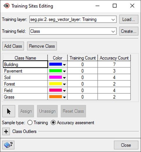
1. On the Object Analyst wizard, under Training Vector Layer, click Edit. The Training Sites Editing window opens.
   • Switch Training Field to Class. The imported ground truth points will be reflected in the Accuracy Count column.
   • For Sample type, choose Accuracy assessment.
     
2. Collect additional accuracy assessment training sites for each class following the steps in Section 4.1 – Selecting training sites.
   
   
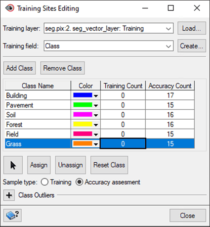
3. When completed, close the Training Sites Editing window.
   

SUPERVISED CLASSIFICATION

Once the training sites are collected, you can run a supervised classification. Supervised classification is a process to find a model, or function, by analyzing the attributes of a data set of which the class memberships are known. This function is then used to predict the class memberships for a target population.

The two supervised classifier methods in the Object Analyst tool are:

1. Support vector machine (SVM) classifier and
2. Random trees (RT) classifier.

OPTIONS FOR SUPERVISED CLASSIFICATION

There are two supervised classifier methods in CATALYST Professional Object Analyst:

Support vector machine (SVM) – a machine-learning methodology used for supervised classification of high-dimensional data. The objective is to find the optimal separating hyperplane (i.e. decision surface, boundaries) by maximizing the margin between classes, which is achieved by analyzing the training samples located at the edge of the potential class.

• Performs better when the training set is small or unbalanced.
• Often requires data to be normalized prior to the training/classification.

Random trees (RT) – a machine-learning algorithms which does ensemble classification. The algorithm uses a set of object samples that are stored in a segmentation-attribute table. The attributes are used to develop a predictive model by creating a set of random decision-trees and by taking the majority vote for the predicted class.

• Unlike SVM, RT can handle a mix of categorical and numerical variables.
• Less sensitive to data scaling.
• Computationally less intensive than SVM and works better and faster with large training sets.

For more information on the classifier methods, click on the CATALYST Help button or search Setting up and running Supervised Classification in in the CATALYST Help.

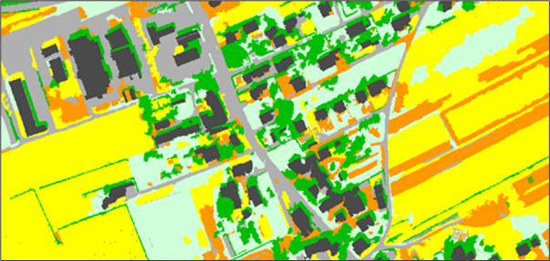
SUPPORT VECTOR MACHINE (SVM) CLASSIFIER

To perform an SVM classification:

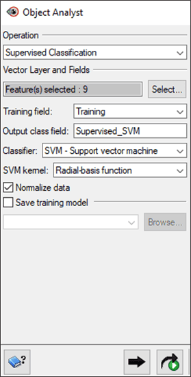
1. In the Object Analyst window, change the Operation to Supervised Classification.
2. In the Vector Layer and Fields section, click Select. The Vector Layer and Field Selector window opens:
   • Ensure the Layer field is populated with seg_vector_layer and that all Fields have a checkmark next to them except Area, Perimeter, and Class_Count.
     
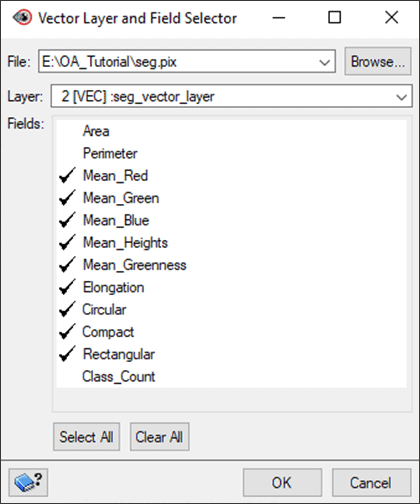
3. Click OK.
4. For Training Field, select Training.
5. In the Output Class Field, change the name to Supervised_SVM.
6. For Classifier, select SVM – Support vector machine.
7. For SVM kernel, select Radial-basis function.
8. Ensure that Normalize Data is checked.
   
   Note: Check Save training model if you wish to preserve the classification routine for use in a Python script.
   
9. Click Add and Run.
10. Once the process has finished, the output will appear in the Process Canvas.
11. In Focus, go to the Maps tab and uncheck the other layers to view your results.
    

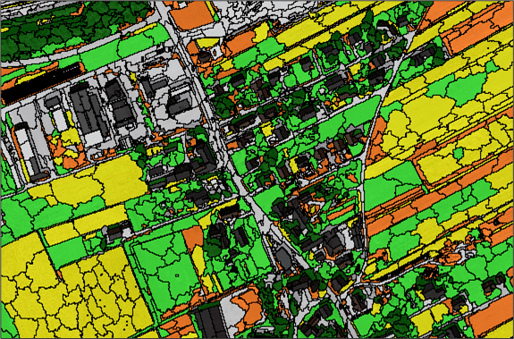
Note: For details on how to adjust the representation of the classes such as removing the borders (as shown below), adjusting the colours, or changing the opacity, go to Section 9 – Post-Classification Editing.

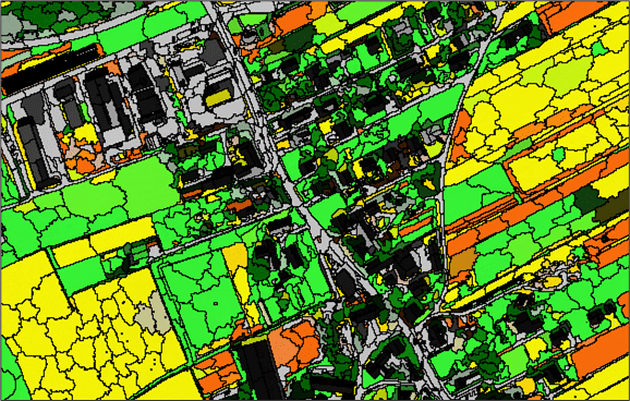
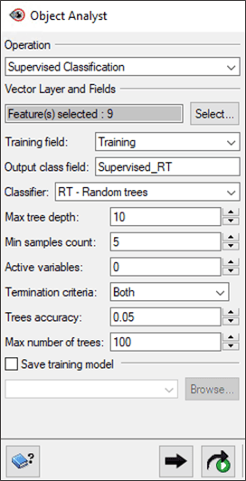
RANDOM TREES (RT) CLASSIFIER

To perform an RT classification:

1. In the Object Analyst window, change the Operation to Supervised Classification.
2. In the Vector Layer and Fields section, click Select. The Vector Layer and Field Selector window opens:
   • Ensure the Layer field is populated with seg_vector_layer and that all Fields have a checkmark next to them except Area, Perimeter, and Class_Count.
3. Click OK.
4. For Training Field, select Training.
5. In the Output Class Field, change the name to Supervised_RT.
6. For Classifier, select RT– Random trees.
7. Leave the default parameters for the rest of the options. For a description of each of the parameters, see the CATALYST Help. 

Note: Check Save training model if you wish to preserve the classification routine for use in a Python script.

9. Click Add and Run.
10. Once the process has finished, the output will appear in the Process Canvas.
11. In Focus, go to the Maps tab and uncheck the other layers to view your results.

Note: For details on how to adjust the representation of the classes such as removing the borders (as shown below), adjusting the colours, or changing the opacity, go to Section 9 – Post-Classification Editing.

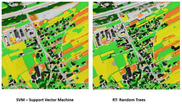
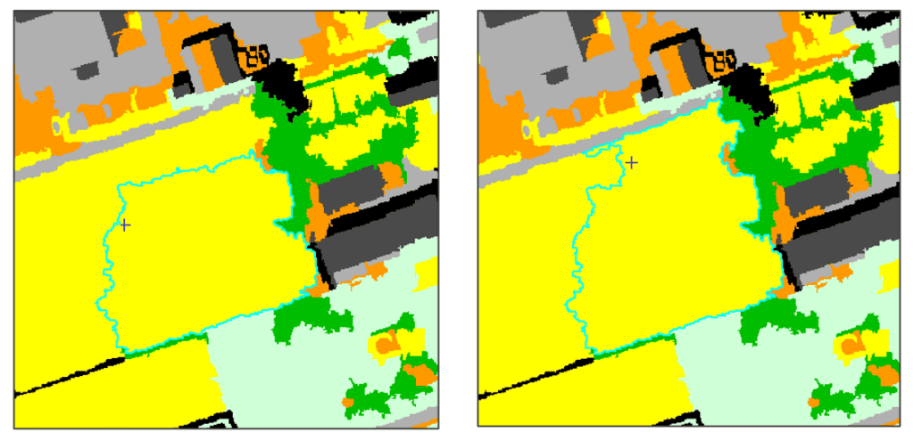
COMPARING RESULTS

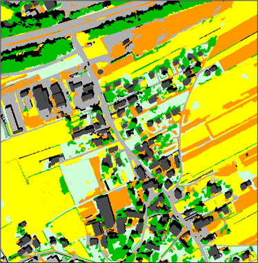
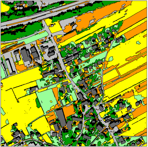
Below is a side-by-side comparison of the results from the SVM (left) and RT (right) classifications. 

UNSUPERVISED CLASSIFICATION

An alternative to supervised classification is unsupervised classification. With an unsupervised classification, training samples are not required. This classification is performed on the selected attributes to find data clusters. Object Analyst provides unsupervised classification based on the k-means clustering algorithm.

Note: In the case of unsupervised classification, you will need to determine which unsupervised classes best correspond to the ground features. If there are multiple ground features included in a single unsupervised class, you can run Rule-Based Classification to create additional classes and reclassify segments.

To perform an unsupervised classification:

1. In the Object Analyst window, change the Operation to Unsupervised Classification.
2. In the Vector Layer and Fields section, click Select. The Vector Layer and Field Selector window opens:
   • Ensure the Layer field is populated with seg_vector_layer and that all Fields have a checkmark next to them except Area, Perimeter, PixelValue, Class_Count, and Supervised_SVM_classlabel.
3. For Output Class Field, change the name to Unsupervised.
4. Under Classifier, change the Clusters value to 7.
   
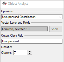
5. Click Add and Run.
6. Once the process has finished, the output will appear in the Process Canvas.
7. In Focus, go to the Maps tab and uncheck the other layers to view your results.

Note: To compare the classifications, reload the supervised classification results to the Maps tab as well. See Symbolizing Classification Results to visualize the information.

ACCURACY ASSESSMENT

An accuracy assessment can be run before or after refining the classification with Rule-Based Classification. Running it before rule-based classification will let us know which classes need to be refined.

To run an accuracy assessment:

1. In the Object Analyst window, change the Operation to Accuracy Assessment.
2. Ensure the Classified vector layer field is populated with the pix file (and seg_vector_layer).
3. Change Classification field to the desired supervised classification.
   • For this tutorial, Supervised_RT is chosen.
4. Change Reference field to Class.
   
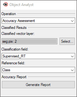
5. Click Generate Report.
6. An Accuracy Assessment Report opens, with the tabs Sample Listing, Error (Confusion) Matrix, and Accuracy Statistics.
7. There are two useful accuracy measures to note:
   1. Error (Confusion) Matrix – Provides details about which training and accuracy sites were classified into each class.
      
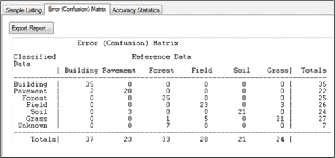
   2. Accuracy Statistics – Provides a range of useful statistics to see how well features were classified.
      

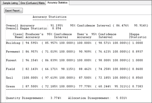
Note: You will notice from our run, that every class had an accuracy result greater than 85%, except for Field. With this information, we can use rule-based classification to adjust this class (See Section 8 – Rule-based Classification for details).

RULE-BASED CLASSIFICATION

In addition to supervised and unsupervised classification algorithms, with Object Analyst you can also create a custom rule to assign class membership to segments. By creating a custom rule, as an analyst you can select the criteria that determines membership of a sample in a class based on your understanding of the domain, data, or both. Either define a rule to assign a class to segments that meet the requirements of the rule, or define a rule to remove the segments from the class.

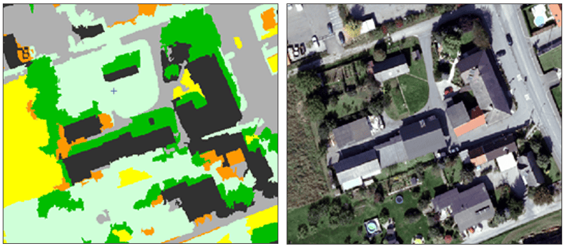
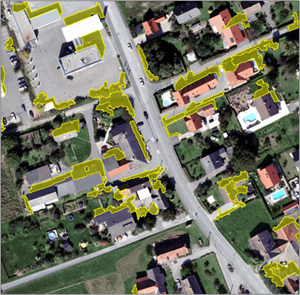
In the Attribute Visualization window of Object Analyst, you can select the vector objects (polygon segments) in the vector layer based on a given attribute (field) and its value range (filter).

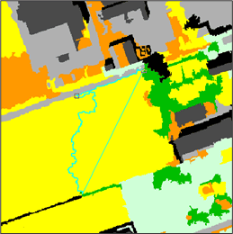
For example, let’s use a rule-based classification to assign the shadow segments to a new Shadow class. In the images below from the supervised classification, notice that the building shadows are part of the forest class (darker green).

To run a rule-based classification:

1. In the Object Analyst window, change the Operation to Rule-Based Classification.
2. For Vector Layer, ensure that seg_vector_layer is selected.
3. For Class Edit, choose Assign.
4. Under Parameters:
   1. For Class field, choose a supervised classification (e.g., Supervised_RT).
   2. For Class filter, choose Forest.
   3. For New class, type Shadow.
5. Check off Specify condition.
   
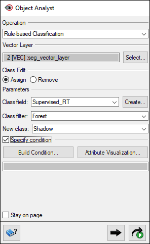
6. Click Attribute Visualization. The Attribute Visualization window opens.
   1. For Class field, choose Supervised_RT.
   2. For Class filter, select Forest.
   3. For Range field, select Mean_Greenness. In the greenness channel, the shadowed areas will be much darker than the actual forest.
   4. Adjust the slider bars. Notice that different segments are selected dynamically. Move the slider bars until enough of the shadow segments are selected. Note: If you set Maximum value too high, you may reclassify too much forest as shadow.
      
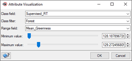
7. Click OK.
   
8. In the Object Analyst window, the condition box will be filled: Mean_Greenness >= 128.1877835083 and Mean_Greenness <= 129.2724260406.
9. Click Add and Run. The shadow class will now be included in your classification.
10. Under the Maps tab, right-click the supervised classification layer and select Representation Editor. You will notice that there is now a new class.
11. Specify a new colour for this class, such as black.
12. On the Representation Editor window, click OK.
    
13. Repeat these steps to reclassify segments from other classes.

POST-CLASSIFICATION EDITING

Once the classification is complete, you may want to modify aspects of your classification. Modifications you can make include the following:

• Merging, splitting, or dissolving polygons,
• Adding new classes, removing existing ones, or reassigning objects of a class, and
• Adjusting style, including border type and opacity.

MERGING AND SPLITTING SEGMENTS

In Object Analyst, there are two methods for merging (and splitting) segments:

1. Automatic dissolve (merging only), and
2. Interactive edits (merging and splitting).

AUTOMATIC DISSOLVE

Automatic dissolve merges two adjacent polygons based on class membership; that is, segments belonging to the same class and that are adjacent to each other are dissolved to create a bigger object. The internal boundaries of such segments are removed. The output will exclude all the attribute fields, except the field that contains the class-membership information. It is this field that is used to dissolve the segments.

To use automatic dissolve:

1. In the Object Analyst window, in the list under Operation, select Post-classification Editing.
2. Under Type, select Automatic dissolve.
3. Under Vector Layer, click Select, and then choose seg_vector_layer.
4. In Class field list, select the field you want – such as Supervised_RT.
5. Set the output file (e.g. output.pix) and layer name (e.g. dissolved_layer).
   
6. Click Add and Run.
7. Load the dissolved layer into the Focus window and update the representation to view the results.
   

INTERACTIVE EDITS

An alternative to Automatic dissolve for reforming shapes is to use Interactive edits. To do so, you must select a layer that contains one or more polygons with class information.

To use Interactive edits:

1. In the Object Analyst window, in the list under Operation, select Post-classification Editing.
2. Under Type, select Interactive edits.
3. Under Vector Layer, select seg_vector_layer.

MERGING SEGMENTS

To merge polygons:

1. Select the Merge Polygon tool .
2. Select a polygon. When you move the cursor over surrounding polygons you will notice that it has changed.
3. Select any surrounding polygons, to merge them with the original polygon.

SPLITTING SEGMENTS

To split polygons:

1. Select the polygon you want to split with the Select tool .
2. Select the Split Polygon tool .
3. Draw a line through the polygon to split it.
   

ADDING, MODIFYING, AND DELETING CLASSES

Classes can be added, modified, and removed, as necessary. You can also assign objects to a class and change the style of how classes are displayed in the view pane.

To add, remove, or modify classes:

1. In the Object Analyst window, in the list under Operation, select Post-classification Editing.
2. Under Type, select Class edit.
3. Under Vector Layer, click Select, and then choose desired layer, such as seg_vector_layer or dissolved_layer.
4. In the Class field list, select the field you want. For this tutorial, the Supervised_RT class is selected.
5. Click Edit. The Class Editing window appears.
6. In this window, add, remove, or update the classes (as detailed below).

Note: This window can also be used to change the representation colour and style for the classes.

ADDING A CLASS

To add a class:

1. Click Add in the Class Editing window.
2. Rename the class.
3. Select the new class from the list.
4. Click the Selection tool and select a segment in the Focus window.
5. Click Assign. The selected segment is now assigned to the new class.
   

REASSIGNING SEGMENTS

To reassign segments to another class:

1. Select the class that you wish to reassign the segments to in the Class Editing window.
2. Select the segment that you wish to reassign. You can select multiple segments at one time.
3. Click Assign. Note: Click Continuously Assign to continue to assign multiple objects that you select to the selected class.
   

DELETING A CLASS

To delete a class:

1. Select a class from the Class Editing list and click Remove.
2. If your class currently has segments assigned to it, you will receive an error. You need to reassign items to another class. Once the class is empty, you can remove it.

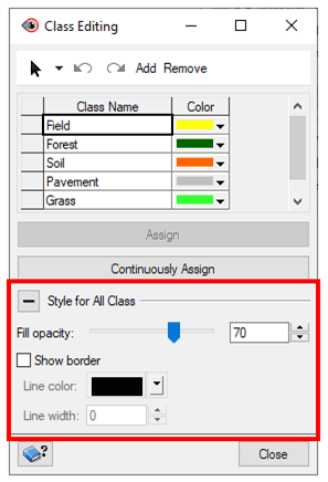
ADJUSTING BORDERS AND OPACITY

The style of the classification can be customized using Style for all Class section of the Class Editing window.

To adjust borders and opacity:

1. In the Class Editing window, expand the Style for All Class section.
2. For Fill opacity, move the slider to increase or decrease the opacity of the polygons.
3. Check or uncheck Show border.

Note: The classification and editing are now complete. At this point, you can rerun Accuracy Assessment to check for an improvement in accuracy.

VIEWING CLASSIFICATION RESULTS

To view the classification results in a Focus window on their own, you must adjust the representation for that layer.

To adjust layer representation:

1. In the Files tab in Focus, right-click seg_vector_layer and choose View.
2. In the Maps tab, right-click the new seg_vector_layer and select Representation Editor.
3. In the Representation Editor window, change the Attribute option to the desired classification field – Supervised/Unsupervised.
4. Click More.
5. For Method, select Unique Values.
6. Ensure Generate new styles is selected and that you choose the style you want to use.
7. Click Update Styles.
8. You can then change the colour of each class in the top section of the panel.