Object Analyst – Batch Classification

The CATALYST Professional Object Analyst is an object-based image-analysis (OBIA) module. It is used to segment an image into objects for classification and analysis. It differs from the traditional pixel-based approach, which focuses on a single pixel as the source of analysis.

BATCH CLASSIFICATION

The Object Analyst workflow has a batch classification feature. With batch classification, you can run classification simultaneously on a collection of images with similar qualities of acquisition. The collection can be any aerial, satellite, or SAR imagery you want classify similarly, such as, but not limited to airphotos (strips or individual images), stacks of historical imagery, overlapping images, or contiguous images.

First, run a classification on an individual image that you want to use as reference image for the batch you want to process. Once the classification results from that image are deemed acceptable, then run a batch classification on the rest of the images to apply the same classification to each. The batch classification applies the following steps:

• segmentation,
• attribute calculation,
• support vector machine (SVM) classification (based on the training-model file you create from the first individual image classified), and
• any number of rule-based classification steps.

More information on each of the steps that are run in this tutorial is included in the online Help Documentation for CATALYST Professional.

THE TUTORIAL DATA

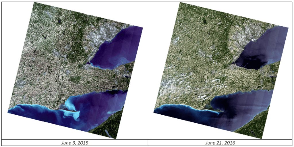
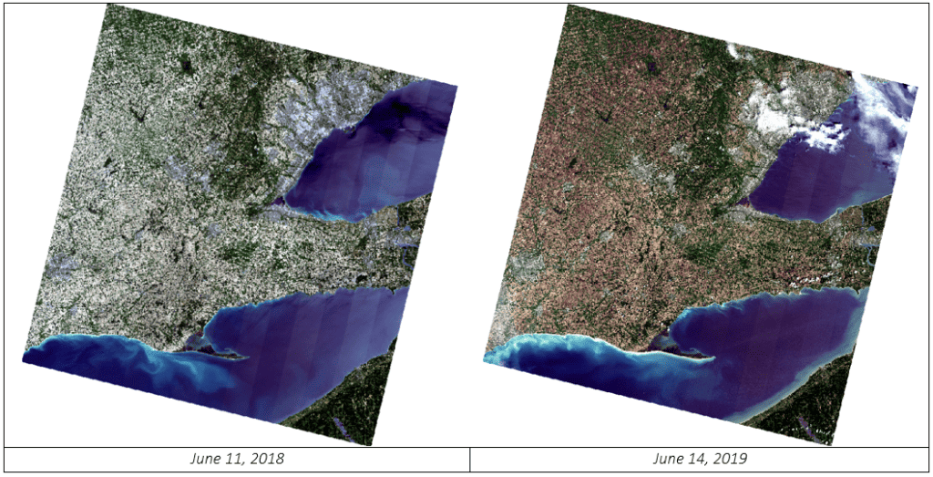
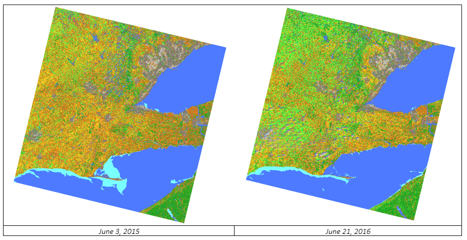
For this tutorial, multi-temporal Landsat-8 data is used, acquired in June over four different years:

1. LC08_L1TP_018030_20150603_20170226_01_T1 – June 3, 2015 (initial image)
2. LC08_L1TP_018030_20160621_20180130_01_T1 – June 21, 2016
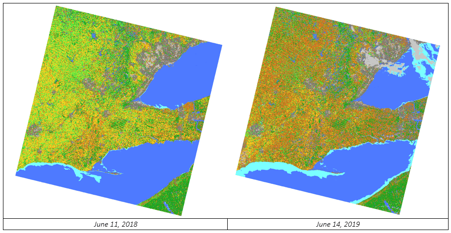
3. LC08_L1TP_018030_20180611_20180615_01_T1 – June 11, 2018
4. LC08_L1TP_018030_20190614_20190620_01_T1 – June 14, 2019

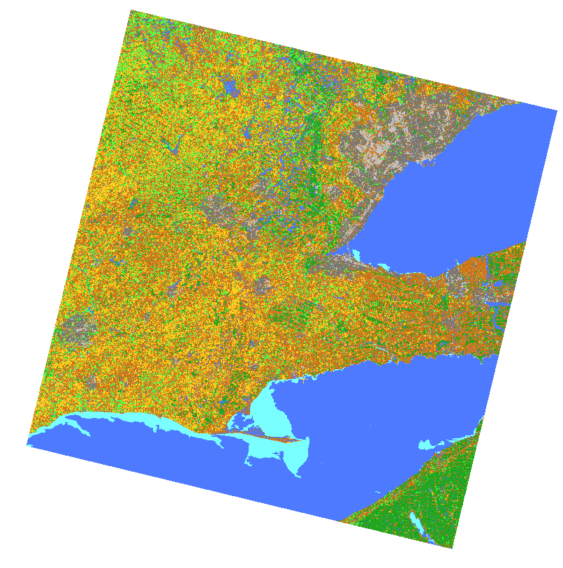
The figures below show the datasets. Notice that two of the batch images include clouds while the initial image does not. 

This factor will be part of the classification exercise. The clouds in those images will be incorrectly classified initially, as there was no cloud class in the initial image classification. After running batch classification, we will run rule-based classification on the two images with cloud to create a new cloud class.

CLASSIFYING THE INITIAL IMAGE

The first step in batch classification is to run the Object Analyst classification on an initial image to use as reference. In this case, we will use LC08_L1TP_018030_20150603_20170226_01_T1 (June 3, 2015) as the initial image. We will run the Segmentation, Attribute calculation and Supervised classification steps. You can also run rule-based classification to edit the classification.

For more information on the workflow for performing Object Analyst classification on a single image, see the Object Analyst tutorial.

Note: Make sure that each of the following steps is completed for the initial image and the Process Canvas in the Object Analyst wizard includes each of the steps that you ran. You will need to reference each step when running a batch classification.

Note: Make sure to continually save your Focus project (.GPR) file when working with Object Analyst. This will ensure all of your steps are saved in the OA Process Canvas.

SEGMENTATION

To run segmentation:

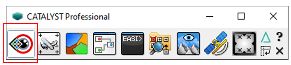
1. Open Focus from the CATALYST Professional toolbar.
   
2. Go to File > Open.
3. Navigate to the Initial_Image folder, select June2015.pix and click Open. The image will automatically load as a true color composite (R:1, G:2, B:3).
4. From Analysis, select Object Analyst. The Object Analyst wizard opens.
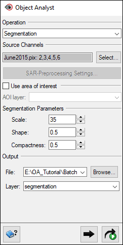
5. For Operation, select Segmentation.
6. For Source Channels, click Select. The Layer Selection window opens.
7. Click Browse, navigate to June2015.pix, and click Open. All the Landsat-8 layers are loaded into the window.
8. Select Layers 2-6.
   
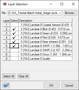
9. Click OK.
10. Under Segmentation Parameters, change Scale to 35 – this will create larger segments then the default of 25.
11. Set Output File name (e.g. 2015_segmentation.pix) and Layer name (e.g. segmentation).
    
12. Click Add and Run .
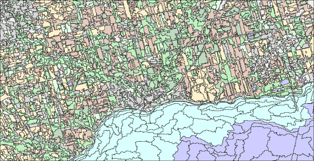
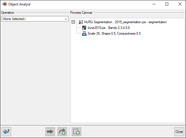
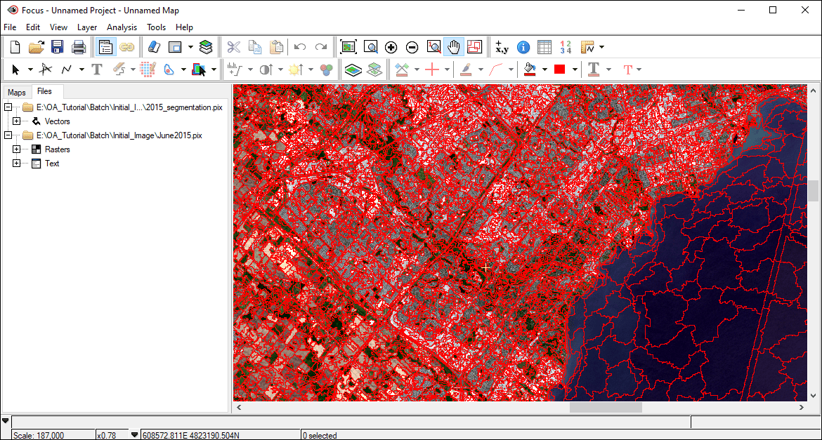
13. After the image segmentation is finished executing, the step appears on the Process Canvas and the new segmentation vector layer will be loaded into Focus.
    
    

ATTRIBUTE CALCULATION

With an attribute calculation, various attributes (e.g. geometrical, statistical, etc.) are computed for each polygon segment, or object.

Note: Each time you set up attribute calculation, Object Analyst uses the same raster channels and segmented vector file as specified for a previous segmentation operation, by default.

To set up and run Attribute Calculation:

1. In the Object Analyst wizard, click on the Operation dropdown list and select Attribute Calculation.
2. Keep the same channels checked off in the Source Channels list.
3. In the Attributes to Calculate section, select Statistical: Mean and Vegetation Indices: NDVI.
   
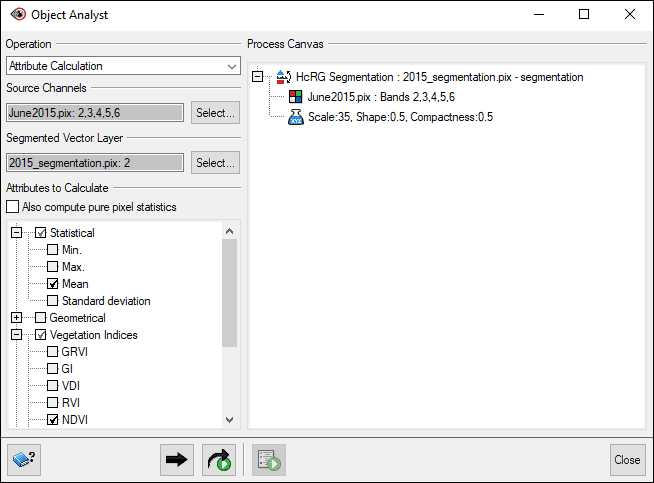
4. Click Add and Run.
5. After the attribute calculation is finished executing, the steps appear on the Process Canvas.

TRAINING SITES EDITING

The next step is to collect training sites used by the learning algorithm to generate the supervised classification model. More detailed training site collection steps are outlined in the Object Analyst tutorial.

To collect training sites:

1. In the Object Analyst wizard, click on the Operation dropdown list and select Training Site Editing.
2. Under the Training Vector Layer section, click Select and make sure that the 2015_segmentation.pix file is selected and segmentation layer is checked off.
   
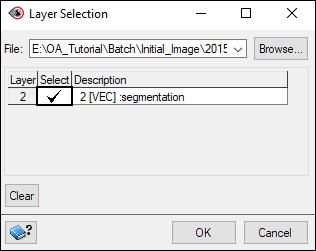
3. Click OK.
4. Click on the Edit button. The Training Sites Editing window opens.
5. Ensure that Training field is set to Training.
6. Click on the Add Class button.
7. A new row will be added that reads Class 1 under the Class Name column.
8. Rename the class with a meaningful name, such as Forest.
9. Adjust colour to a meaningful value (i.e., Forest > Green, Water > Blue).
10. Click on the Individual Select tool .
11. In the Focus viewer, zoom in to a section of the image, hold the CTRL key down, and select the segmentation polygons that match the current class (i.e., Forest). Try to be as accurate and diverse in your collection as possible.
12. Once you’ve selecting at least 20-30 sites, click Assign.
    
    Note: To unselect the polygons from the previous class once you are moving on to a new class, click any new polygon without the CTRL key pressed.
    
    Note: To better inspect the imagery, toggle the segmentation layer on and off.
    
    
13. Continue to add new classes and collect training sites so that you have similar classes to the screenshot below.
    
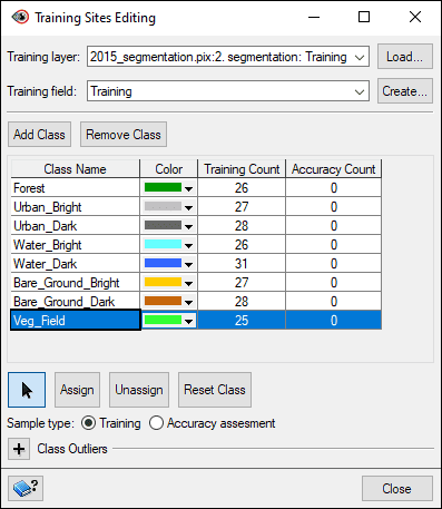
14. Click Close.
    

SUPERVISED CLASSIFICATION

Now that the training sites are collected, the next step is to run the supervised classification.

To run a supervised classification:

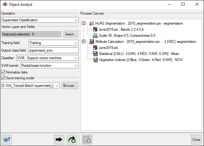
1. In the Object Analyst wizard, change the Operation to Supervised Classification.
2. Under the Vector Layer and Fields section, click on the Select button. The Vector Layer and Field Selector window opens.
3. Make sure that the File field is populated with the 2015_segmentation.pix file, and the Layer field is populated with the segmentation layer. Make sure the five Mean fields and NDVI are selected.
   
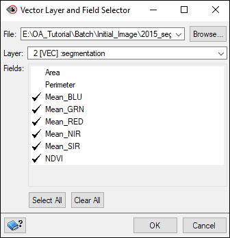
4. Click OK.
5. In the Training Field dropdown list, select Training.
6. In the Output class field, change the name to supervised_svm.
7. Leave the Classifier as SVM – Support vector machine and SVM kernel as Radial-basis function.
8. Check off Save training model and set an output location and name for the training model .TXT file, e.g. supervised_training_model.txt.
   
   Note: The SVM training model created in this step is used in the batch classification later in the tutorial. The supervised classification uses training samples and object attributes, stored in a segmentation attribute table, to create a series of hyperplanes, and then writes them to an output .TXT file as the SVM training model.
   
9. Click Add and Run .

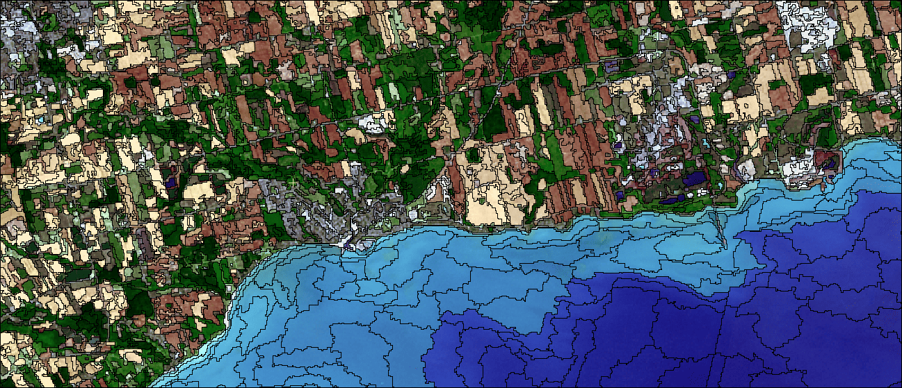
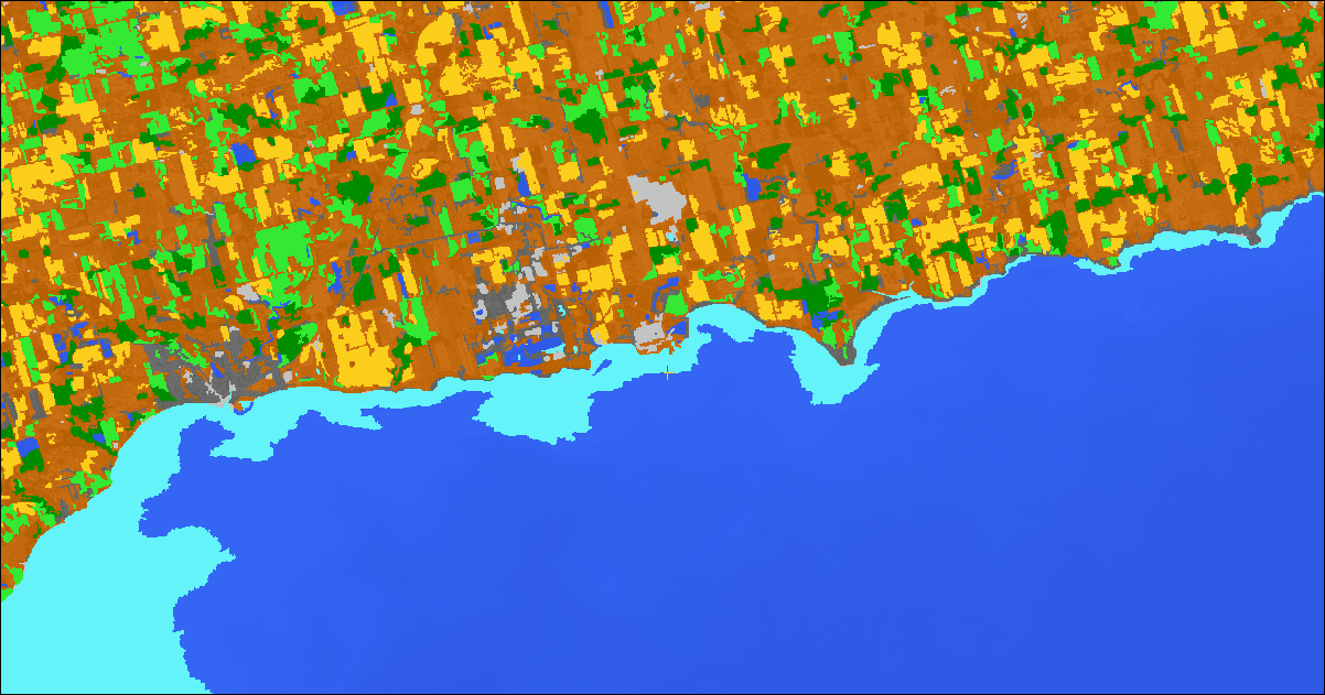
Once the classification is complete, you can view the result in Focus. The classification is loaded using the colours that you specified in the training site editor. Toggle the image layer to view the classification segments on their own.

EDITING REPRESENTATION (OPTIONAL)

If desired, you can edit the classification representation for the segmentation layer.

To edit the representation:

1. In the Object Analyst wizard, change the Operation to Post-Classification Editing.
2. Under Type, choose Class edit.
3. Under Vector Layer, click Select. The Layer Selection window opens.
4. Choose your segmentation file and layer, segmentation. Click OK.
5. Set Class field as supervised_svm.
   
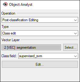
6. Click Edit. The Class Editing window opens.
7. Expand the Style for All Class section.
8. Adjust the classification colours, opacity, and select whether to show borders, as desired. For this tutorial, Fill opacity was changed to 87% and Show border was unselected.
   
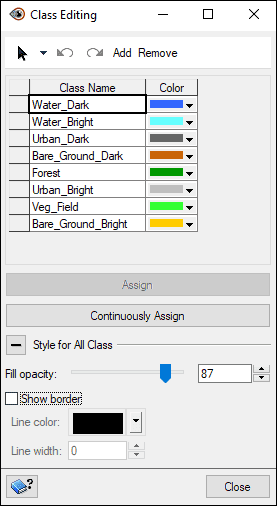
9. Click Close.
   
   
10. Close the Training Sites Editing window.

Note: For your Accuracy Count, you have the option to either:

• repeat the steps above to manually collect validation sites, or
• Import Ground Truth Points as explained in the section below.

SAVING REPRESENTATION TO RST FILE

In order to apply the same representation to various files, save it to a system-linked representation style table (RST) file.

To save the representation to an RST file:

1. In Focus, in the Maps tab, right-click the new vector layer, supervised_svm, and choose Representation Editor. The Representation Editor window opens.
2. To save the representation, click Save . The RST Save As window opens.
3. Under Output, choose a File name, e.g., rep_batch_class.rst.
   
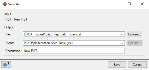
4. Click Save.
5. Click OK on the Representation Editor window.

Note: This is a good time to save your Focus project file.

ADDING RULE-BASED CLASSIFICATION (OPTIONAL)

If you need to further refine the classification on the initial image you can run rule-based classifications. For this tutorial, rule-based classifications are not added at this stage. Instead, they are created and run on specific images after the batch classification.

For more information, click on the CATALYST Help button or search Rule-Based Classification in the CATALYST Help.

More details on Rule-Based Classification are also outlined in the Object Analyst tutorial.

RUNNING BATCH CLASSIFICATION

The initial image has been successfully classified, so now we can run a batch classification on the additional images.

To run a batch classification:

1. In the Object Analyst wizard, change the Operation to Batch Classification.
2. For Input Images, set Folder to the folder containing your additional images. For this tutorial, choose the folder Additional_Images. If required, you can change the Search pattern (but in our case we will search for .PIX files).
3. For Output Folder, set to the folder where you wish to save the output segmentation files containing the classification information, e.g. Output.
4. For Training Model, select the TXT file you saved in the Supervised classification step, supervised_training_model.txt.
   
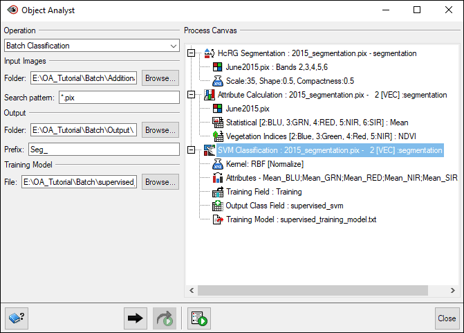
5. Click Add .
6. The Batch Classification process is added to the Process Canvas. Under Batch Classification, the Segmentation, Attribute Calculation, and SVM Classification items are each displayed in red. This indicates you must complete the definition of each before running the batch classification.
   
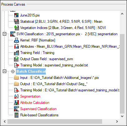
7. In the Process Canvas box, find the segmentation process you want to use. In this case, we will use the HcRG Segmentation process at the top of the pane. Right-click the process, select Add To > Batch Classification.
   
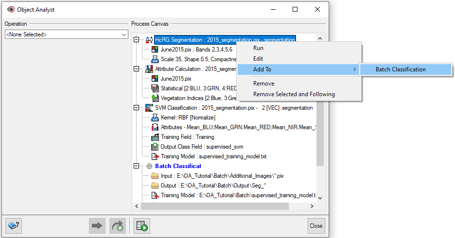
8. The Batch Classification process is updated with the segmentation process you added.
9. In the same manner, add the Attribute Calculation and SVM Classification processes.
   
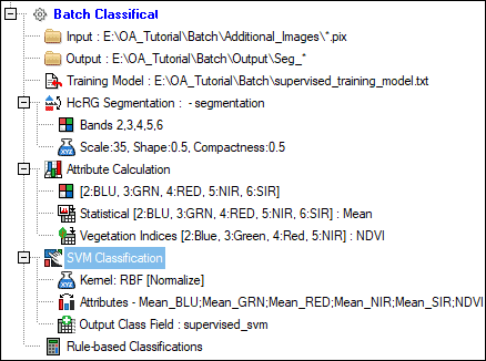
10. The Batch Classification process is now ready to run. In the Process Canvas, right-click Batch Classification and select Run.
11. A progress window is displayed, showing the status of the segmentation, attribute-calculation, and classification steps for each input image. The new segmentation files are saved to the output folder.
    
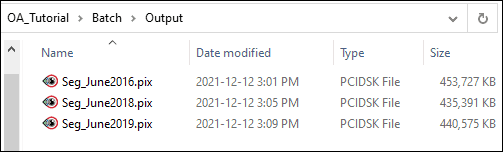
12. Once the processing is complete, open the various segmentation PIX files in Focus to view the segments and classification information.
    
    The next section outlines how to apply the saved RST file to each of the new segmentation layers.

APPLYING REPRESENTATION TO ADDITIONAL LAYERS

When you load the additional classifications to Focus as vector layers, you want to ensure that the RST file you created is linked to the map in your project.

To apply representation to additional vector layers:

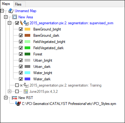
1. In Focus, under the Maps tab, right-click on Unnamed Map and select Representation > Load.
2. Select the RST file that you created in the Saving representation to RST file step, called rep_batch_class.rst, and click Open.
3. The RST file will now be listed in the Maps tab.
   
4. Open the additional segmentation files in Focus.
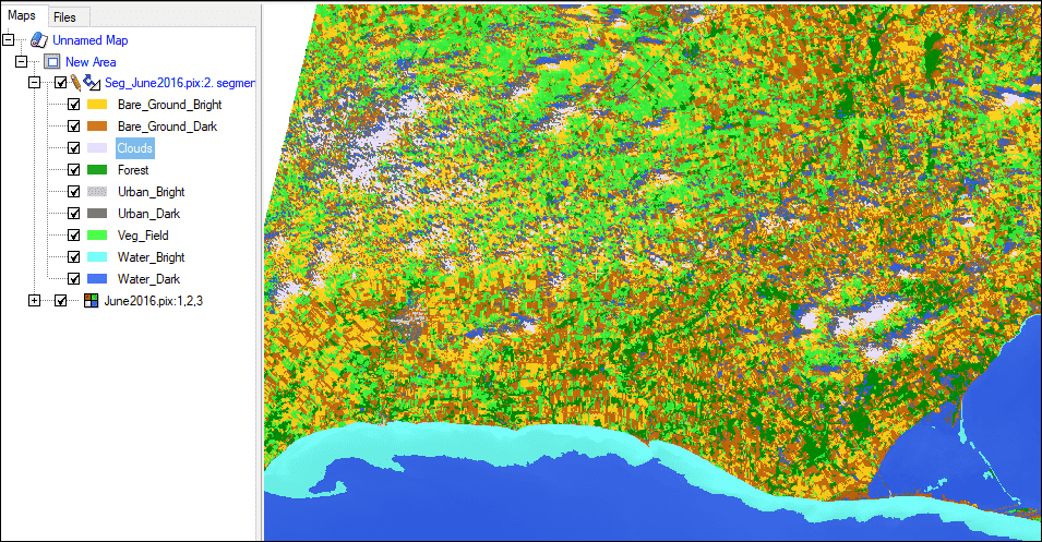
5. Under the Maps tab, right-click on the top new vector layer, Seg_June2016.pix, and select Representation Editor. The Representation Editor window opens.
6. Change the Attribute drop-down menu to the supervised_svm field and click OK.
   
7. The representation from the RST file will be applied.
8. Apply the RST to the other segmentation vector layers in the same manner.

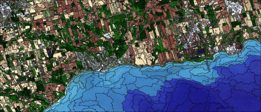
POST CLASSIFICATION EDITING

To further refine the classification after completing a batch classification, you can run a rule-based classification. To illustrate this, we will add a cloud class. We did not initially specify one, but clouds become a more significant class in other images, as can be seen over the water in June2019.pix.

Example of post-classification editing: Adding a cloud class

For the tutorial, we will re-run an attribute calculation on the June2016 image to calculate the Max_CIR value in order to better differentiate clouds from other features. This attribute is the maximum value from the Cirrus band that Landsat-8 provides.

Then we will run a rule-based classification on the June2016 image to reclassify the clouds that were incorrectly classified as Urban_bright as a new class called ‘Clouds’. You can also perform similar steps to reclassify the clouds in other images.

RE-RUNNING ATTRIBUTE CALCULATION

To re-run Attribute Calculation:

1. In a new Focus window, open June2016.pix and Seg_June2016.pix.
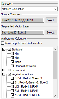
2. Open the Object Analyst wizard, click on the Operation dropdown list and select Attribute Calculation.
3. For Source Channels, click Select. The Layer Selection window opens. For File, choose June2016.pix.
4. All the Landsat-8 layers are loaded into the window.
5. To include Cirrus clouds, select Layers 2-6 and 8.
   
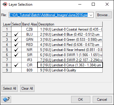
6. Click OK.
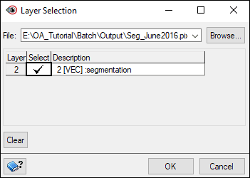
7. For Segmented Vector Layer, choose Seg_June2016.pix. Click OK.
8. In the Attributes to Calculate section, as before, select Statistical: Mean and Vegetation Indices: NDVI. Now also select Statistical: Max to include the Max CIR value.
   
9. Click Add and Run .
10. After the attribute calculation is finished executing, the steps appear on the Process Canvas.

RUNNING RULE-BASED CLASSIFICATION

To run a rule-based classification:

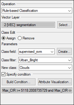
1. In the Object Analyst wizard, click the Operation dropdown and select Rule-based Classification.
2. For Vector Layer, click Select. The Layer Selection window opens. Make sure that the file is Seg_June2016.pix and the segmentation layer is selected.
   
3. Under Parameters:
   • For Class Edit, keep as Assign.
   • For Class field, choose supervised_svm.
   • For Class filter, choose Urban_Bright.
   • For New Class, type Clouds into the field.
   • Check off Specify Condition and click Attribute Visualization. The Attribute Visualization window opens.
4. In the Attribute Visualization window:
   • For Class field, choose supervised_svm.
   • For Class filter, choose Urban_Bright.
   • For Range field, choose MAX_CIR.
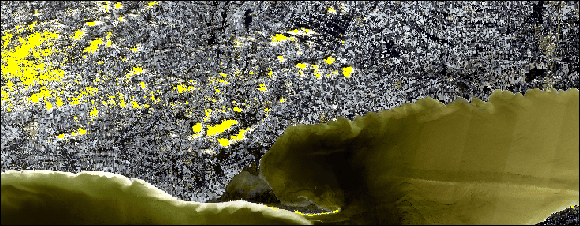
   • Adjust the sliders to select segments which contain clouds. Segments that contain MAX_CIR values within the specified range will be highlighted as yellow and change dynamically as you play with the range.
     
     
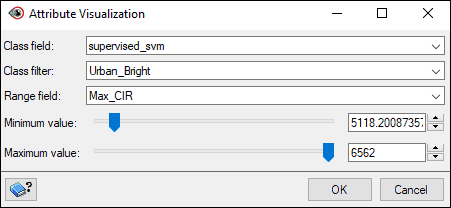
   • Once you are satisfied, click OK.
     
5. Click Add and Run. The Rule-based classification runs to reclassify those selected segments to the new Cloud class.

APPLYING TO OTHER IMAGES

Once the Cloud class has been added to June2016.pix, you can take additional steps to style the class and apply it to other images, if desired.

To style the class and apply it to other images:

1. Once the rule-based classification is complete, adjust the representation style of the new class, if desired (see the Section “Editing representation”).
   
2. Save the representation to an RST file to run a new batch classification on all the images with clouds (see Sections “Saving representation to RST file” and “Running batch classification”).