
You can use the EASI scripting language to write scripts and run them on data you have open in Focus. You can also open the EASI Modeling window to run EASI scripts for data that is not open in Focus. Dozens of pre-written scripts are available in the CATALYST Professional pro folder - C:\PCI Geomatics\CATALYST Professional\pro
For details on numeric, string, logical, and modeling (channel, bitmap and special variable) expressions, see the EASI topic in the CATALYST Professional Help.
EASI Modeling in Focus operates on a single input file, which you select from the drop-down list in the Modeling window. The basic steps required to run a simple model are outlined below. Note that the model is performed directly on the database file. It is highly recommended you backup the input file before the model is run. You can also test the model using bitmaps instead of image layers where applicable.
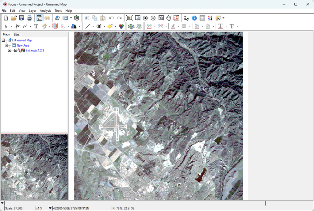
1.1 Open PIX file in Focus – File > Open (A model can be run on any PIX file. It does not have to be displayed in the Focus viewer). The image and bitmap layers must exist in the database PIX file prior to running the model. To add the required image and bitmap layers to a PIX file loaded in Focus, right mouse click on the file in the File Tab and select New > Image Layer (or Bitmap Layer).
1.2 Load an existing bitmap layer (if required). Right mouse click the Area on the Map Tab and select Add Layer > Bitmap.
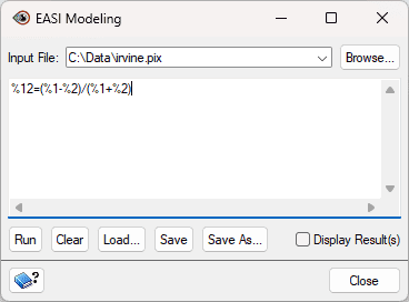
1.3 Open EASI Modeling Window –“Tools | EASI Modeling”
• Select “Input File” from drop-down list
• Enter Model in text editor
• Run – execute the displayed model
• Clear – delete displayed model
• Load – load an existing model (.EAS extension)
• Save – save model to text file (.EAS extension)
• Check box "Display Result(s) – display results in Focus Viewer
The Modeling window provides the option of displaying the results to the Focus viewer. It is not necessary to save this new layer back to the database as the Modeling program operates on the database file itself, rather than the display. Once you have reviewed the results on-screen, you can simply delete the new layer - right mouse click on the layer under the Map Tab and select "Remove". For more details on EASI Modeling expressions, launch the context sensitive help from the Focus EASI Modeling window and select "Expressions". This will provide more details on numeric, string, logical and Modeling (channel, bitmap and special variable) expressions. The on-line help provides details on the entire EASI scripting language. EASI Modeling in Focus is designed primarily for simple image Modeling. While all options are available for PACE MODEL scripts run at the EASI prompt, only a subset of these commands can be used in the Focus EASI Modeling window.
Modeling equations in their simplest form are arithmetic combinations of image layers assigned to other image layers. Image layers are indicated by a percent sign followed by the layer number. The following equation assigns the average numeric value of image layers 1 and 2 to image layer 3.
%3 = (%1 + %2)/2
The assignment is evaluated for every pixel in image layer 3, using the corresponding pixel values from image planes 1 and 2.
You can also assign a constant value to an entire image layer.
%1 = 255
A standard set of arithmetic operations is available in Modeling expressions:
a + b Addition
a - b Subtraction
a * b Multiplication
a / b Division
a ^ b Exponentiation
( a ) Parentheses, also square brackets [].
- a Unary negation
A wide set of mathematical intrinsic functions are also available, including the sin(), cos(), tan(), asin(), acos(), atan(), ln(), log10(), exp(), exp10(), rad(), deg(), abs(), int(), random() and frac() functions.
All the rules previously indicated for image layers also apply to bitmap layers, except that the variables are prefixed with two percent characters instead of one. A bitmap layer can have a value of either 1 (ON) or O (OFF). For example, if image layer 1 has a digital number greater than 50, then set bitmap layer 15 to 1.
If %1 > 50 then
%%15 = 1
endif
In addition to simple assignment equations, it is also possible to construct simple logical operations in the Focus Modeling command window. These operations take the form of "IF" statements.
The following command would set the numeric value of image layer 2 to 255 anywhere the value of image layer 1 is between 32 and 64. Note that line breaks are significant - each statement must be on its own line.
if (%1 >= 32 AND %1 <= 64) then
%2 = 255
endif
This more complex example shows a procedure to turn on bitmap layer 2 (%%2) where image layers 1, 2, and 3 all are equal to 255.
if (%1 = 255) and (%2 = 255) and (%3 = 255) then
%%2 = 1
else
%%2 = 0
endif
The possible comparison and logical functions are:
a > b a greater than b
a < b a less than b
a = b a equals b
a <> b a not equal b
a <= b a less than or equal b
a >= b a greater than or equal b
a OR b a is true or b is true
a AND b a is true and b is true
!a a is not true
It is also possible to use brackets to ensure operations take place in the expected order.
The example below performs a vegetative index calculation using image layers 1 and 2 and saves the result to image layer 12.
Add a 32 bit real image layer to irvine.pix to store the results.
On the Focus File Tab – Right-click on Irvine.pix – “File | New | Image Layer“
%12 = (%1-%2)/(%1+%2);
To output to an 8-bit image layer, some scaling and adjustment is necessary:
%8 = ((%1-%2)/(%1+%2))*128 + 127.5;
Add a bitmap layer to irvine.pix: – File Tab – Right-click on irvine.pix – New > Image Bitmap Layer.
To view the results in the Focus viewer, check the "Display Results" box or add the new bitmap layer to the Map Area – Map Tab –Right Click on Area – Add > Bitmap
if (%1 < 55) and (%2 < 55) and (%3 < 55) then
%%33 = 1
else
%%33 = 0
endif
Note: The demo file irvine.pix does not contain a black "no data" area outside the image so the purpose of this example a digital number of less than 55 in image layers 1, 2 and 3 was used to create the bitmap layer. If you were creating an actual mask for the “no data” area you would use (%1 = 0) and (%2 = 0) and (%3 = 0) in the IF statement.
Change area under bitmap to white in image layers 1, 2, and 3;
if %%29=1 then
%1=255 %2=255
%3=255
endif;
if (mod(@geox,1000)<=@sizex) or (mod(@geoy,1000)<=abs(@sizey)) then
%1 = 255
%2 = 255
%3 = 255
else
%1 = %1
%2 = %2
%3 = %3
endif
Please refer to the “Special Variables” section below for details on the use of @geox/ @geoy & @sizex/ @sizey.
Create an image which smoothly blends image layer 1 into image layer 2 as you move across the image. The output is placed in image layer 8.
%8 = ((@x-1)/@dbx)%2 + ((@dbx-@x)/@dbx)%1
%8 = ((@x-1)*255) / @dbx
Note the use of backslashes to extend a statement over multiple lines. Also note that Algorithm Librarian program FAV performs this operation more efficiently.
%8 = (%4[@x-1,@y-1] + %4[@x,@y-1] + %4[@x+1,@y-1] + \
%4[@x-1,@y ] + %4[@x,@y ] + %4[@x+1,@y ] + \
%4[@x-1,@y+1] + %4[@x,@y+1] + %4[@x+1,@y+1] ) / 9
When processing pixels on the border of the image, the neighborhood of the current pixel will extend off the database. To ensure that referenced pixels that are off the database (such as %4[@x-1,@y-1] in the top left corner) are usable the image values are replicated out from the edge of the database to supply values that are missing.
The following section describes EASI Modeling syntax in more detail.
Image Layers may be specified in a modeling expression using any of the following forms:
%n [(x_expr, y_expr)]
%{ n } [(x_expr, y_expr)]
%{ file_spec, n } [(x_expr, y_expr)]
The first case is the image layer sign (%) followed by literal numeric value such as 1, 2 or 3, indicating layer 1, 2 or 3 of the implicit database (i.e. the input file). The second example is similar, but the image layer number may be a numeric expression that is evaluated to be the image layer number.
The third case is more general yet. The file_spec may be a database file name or a file handle returned by DBOpen(), and the image layer number is evaluated as an expression("n").
Note that for simple models, you cannot reference files other than the input file selected from the drop- down list. EASI Modeling in Focus generally operates on a single file for both input and output. For example, you cannot not run the following model if your input file is "C:\PCI Geomatics\CATALYST Professional\demo\irvine.pix”:
%12 = %{"C:\Geomatica_V100\demo\eltoro.pix", 1}
However, you can override this by using the DBOpen() function to open any number of database files. To copy image layer 1 from eltoro.pix to image layer 12 in irvine.pix:
local integer fdinput, fdoutput
fdinput = DBOpen( "C:\PCI Geomatics\CATALYST Professional\demo\eltoro.pix", "r") fdoutput = DBOpen( "C:\PCI Geomatics\CATALYST Professional\demo\irvine.pix", "r+")
%{fdoutput,12} = %{fdinput,1}; call DBClose(fdinput)
call DBClose(fdoutput)
Note that irvine.pix file is 512x512 and eltoro.pix is 1024x1024. The previous operation copies image layer 1 of eltoro.pix to image 12 of irvine.pix, but because irvine.pix is the implicit database (i.e. the input file), the area of operation is 0, 0, 512, 512 and so only the top left quarter of eltoro.pix is copied into channel 12 of irvine.pix.
The second part of the image layer specification is the subscript specification which is optional. In the above case, the default subscript specification was used which is x --> x, y --> y. The subscript specification allows you to indicate the pixel that should be operated on for the current value of X and Y and may be given as an expression.
The following example is similar to the last, but actually assigns a sampled copy of eltoro.pix to irvine.pix. The @x and @y symbols are the current pixel location when the expression is evaluated for each pixel.
local integer fdinput, fdoutput
fdinput = DBOpen( "C:\PCI Geomatics\CATALYST Professional\demo\eltoro.pix", "r") fdoutput = DBOpen( "C:\PCI Geomatics\CATALYST Professional\demo\irvine.pix", "r+")
%{fdoutput,12} = %{fdinput,1}(@x2+1,@y2+1); call DBClose(fdinput)
call DBClose(fdoutput)
In the above expression, X and Y vary from 0 to 511 as the implicit window of operation is 0, 0, 512, 512 … the area of irvine.pix. However, image layer 1 of eltoro.pix is sampled for values of 1 to 1023. As @x and @y value from 0 to 511, the expression @x*2+1 varies from 1 to 1023. It is also legal for the subscript expressions to extend of the source database. In this case image values from the edge of the database are replicated out as far as is needed to satisfy requests. Thus, a simple filter such as example 4.6 above will work in a reasonable manner, even on the edge of the database.
Bitmaps layers are basically one bit deep image layers used primarily to serve as masks for regions where operations are to take place and may be specified in a manner very similar to image layers. All the rules previously indicated for image layers also apply to bitmap layers, except that the variables are prefixed with two percent characters instead of one. Also, the index number is the segment number of the bitmap layer to be used.
%%n [(x_expr, y_expr)]
%%{ n } [(x_expr, y_expr)]
%%{ file_spec, n } [(x_expr, y_expr)]
Bitmap layer variables will only assume values of zero or one. Any non-zero value assigned to a bitmap layer will be treated as one.
Example: Create a bitmap mask (segment 2) which is true (1) everywhere channels 1 and 2 are less than 25. Then this mask and the mask in segment 3 are used to determine a region that should be zeroed in image channels 1 and 2.
if( %1 < 25 and %2 < 25 )then
%%2 = 1
else
%%2 = 0
endif
if ( %%2 = 1 and %%3 = 0 )then
%1 = 0
%2 = 0
endif
Special variables allow access to information about the size and georeferencing information of channels being operated on, as well as the position of the current pixel. The following special variables may be treated as elements in modeling expressions.
@x current x (pixel) processing location
@y current y (line ) processing location
@dbx size of database in x (pixel) direction
@dby size of database in y (line ) direction
@meterx size of a pixel in x direction in meters
@metery size of a pixel in y direction in meters
@geox x georeferenced centre of current pixel
@geoy y georeferenced centre of current pixel
@sizex x size of a pixel in georeferenced units
@sizey y size of a pixel in georeferenced units
Note that @x, @y, @geox and @geoy change value for each pixel processed, while @dbx, @dby, @meterx, @metery, @sizex and @sizey remain constant over the whole image. It is usually necessary to use the @x and @y special variables when constructing subscript expressions for channel expressions.
For example, the following assignment would mirror an image across a vertical centre line. The @dbx is used in computing the centre line.
%2 = %1[@dbx-@x+1,@y]
Numeric expressions in EASI are normally operated on in double precision floating point. Values with less precision are promoted to double precision before operations are performed. A wide set of built-in operations are available in numeric expressions. They are listed below accompanied by a short description.
a + b Addition
a - b Subtraction
a * b Multiplication
a / b Division
a ^ b Exponentiation
( a ) Parentheses, also square brackets [].
- a Unary negation
A numeric element can be any of the following:
• A numeric constant.
• An EASI variable of type byte, int, float or double.
• An element of a numeric variable array.
• A numeric intrinsic function.
• A numeric user defined function.
• A subscripted numeric parameter
Numeric constants can be entered as decimal or scientific notation numbers with an optional negative sign. Scientific notation is denoted with the "E" or "D" character - for example 123000 can be written as 1.23e5, , 1.23 * 10 ^ 5
a > b a greater than b
a < b a less than b
a = b a equals b
a <> b a not equal b
a <= b a less than or equal b
a >= b a greater than or equal b
a OR b a is true or b is true a AND b a is true and b is true
!a a is not true
Example:
if (%1 = 255) and (%2 = 255) and (%3 = 255) then
%%2 = 1
else
%%2 = 0
endif
Logical expressions in EASI are used to compute TRUE/FALSE results for use with the IF and WHILE conditional statements. There is currently no way to store a pure logical value in an EASI variable. Logical expressions consist of comparisons between numeric and string expressions combined with the use of the logical operations AND, OR, and NOT.
The equality and inequality tests may be used with two numeric expressions. The equal sign ("=") is used to test for equality, while inequality is tested with "<>" or "!=".
Examples:
If( %1 = 0 ) then
…
while( flag <> 1 )
…
The ">", "<", ">=" and "<=" operations may only be performed on numeric expressions. Examples: while( total <= 100 ) while( total < 101 ) while( NOT total > 100 ) while( NOT total >= 101 )
The logical operations AND and OR operate on two logical expressions, while NOT operates on one logical expression. The symbols "&", "|" and "!" are considered to be equivalent to AND, OR, and NOT.
Examples:
if( A = 1 AND B = 1 )then
…
endif
if( A = 1 & b = 1 )then
… endif
IF
The IF statement is used to conditionally execute statements.
IF( logical_expression )THEN statement_list
[ELSEIF( logical_expression )THEN
statement_list] [ELSE
statement_list] ENDIF
logical_expr - A logical expression as described in the Logical Expression topic. statement_list - A list of one or more statements.
Each logical_expression is evaluated in turn until one of them evaluates to be true. When one is true, the corresponding statement_list will be executed, and control will continue beyond the ENDIF. If none of the logical expressions is true and an ELSE clause exists, the associated statement_list will be executed.
The EASI WHILE command provides a general purpose looping construct.
WHILE( log_expr ) statement_list
ENDWHILE
log_expr - a logical expression which is evaluated before each iteration of the loop.
The logical expression in the WHILE statement is evaluated and if the result is true, the statement list is executed; otherwise, control skips to the statement following the ENDWHILE. After the statement list has been executed, control returns to the WHILE statement to test the logical expression again. It is possible to jump into, or out of, the WHILE loop using the GOTO statement, but this is poor style and may not work in future versions of EASI.
The EASI FOR command provides a simple looping construct over a series of numeric values.
FOR iter_var = start_val TO end_val [BY incr_val] statement_list
ENDFOR
iter_var - The iteration variable. This may be any numeric variable type, including a parameter.
start_val -This initial value to assign to the iter_var'.
end_val -Wheniter_var' passes this value, iteration stops.
incr_val - Value by which to increment iter_var' each iteration. The default is1'.
The FOR statement initializes the iteration variable to the initial value, checks it against the end value, and if the end value is not exceeded it executes the statement list. When the ENDFOR statement is reached, the iteration variable is increased by the increment value and compared to the end value. If the end value is not exceeded, the statement list is executed again.
The start value may be greater than the end value and the increment value may be negative, but if the increment value does not take the iteration variable value closer to the end value each iteration, the FOR loop will never terminate. It is possible to alter the value of the iteration variable inside the FOR loop and also to use GOTO's to escape or enter the loop, but this is poor style and may cause problems in future versions of EASI.
Example:
The following example runs the PACE task CLR on the first 128 channels of the PCIDSK file irvine128.pix in groups of 16 channels at a time.
local i,j valu = 0
file="C:\PCI Geomatics\CATALYST Professional\demo\irvine128.pix” for i = 1 to 128 by 16
for j = 1 to 16 dboc(j) = i + j - 1
endfor run clr
endfor
Multiple statements can be placed on the same line by separating the statements with a statement separator. The backslash and semi-colon characters can be used interchangeable for this purpose. A line of input may be almost any length.
Examples:
File = "C:\PCI Geomatics\CATALYST Professional\demo\irvine.pix" \ run clr File = "C:\PCI Geomatics\CATALYST Professional\demo\irvine.pix"; run clr
Single Statements on Multiple Lines
You can split very long statements over multiple lines by placing a backslash character, but not a semi-colon at the end of each incomplete line.
Example:
this_string = one_long_string + a_second_long_string + \ another_long_string + a_really_long_long_string + \