The Atmospheric Correction wizard provides users with the easiest and fastest way to perform a variety of atmospheric corrections. The wizard automatically populates most of the required parameters using the image metadata and guides the user through each step. This tutorial outlines the atmospheric correction workflow including the Interactive Cloud Masking and Interactive Spectral Plot tools. More information about the ATCOR workflow is available from the Help documentation (Contents Tab > Geomatica Help >Focus >Atmospheric Correction).
In this tutorial atmospheric correction is being performed on Landsat-8 Imagery which is available online from the Earth Explorer website: http://earthexplorer.usgs.gov/
1.1. Open Focus from the Professional toolbar.
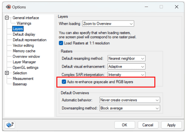
1.2. Turn Auto Re-enhance on:
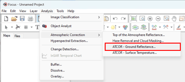
1.3. Open the ATCOR-Ground Reflectance window: select Analysis > Atmospheric Correction > ATCOR – Ground Reflectance
1.4. The Atmospheric Correction panel opens and contains 4 standalone workflows that can be run independently of one another. The four workflows are:
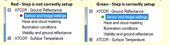
The ATCOR wizard is equipped with indicator symbols that indicate to a user that a given step in the workflow is correctly setup and the user can proceed to the next step.
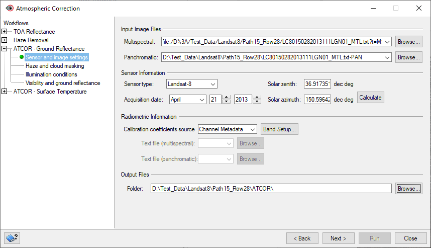
1.5. Select the Sensor and image settings step in the ATCOR – Ground Reflectance workflow.
2.1. Click browse beside the multispectral box and select the MTL file from the Landsat-8 dataset. A box will appear with the options PAN, MS, Thermal, and Quality. Choose MS (Multispectral).
Note: The _MTL.txt file must be used for inputting the imagery as this file contains all of the required metadata for further processing. When working with other sensors, choose the appropriate key file for your data. More information is found in the Help documentation.
2.2. You can also choose to add a panchromatic band to the Panchromatic box using the same method as above but choosing PAN.
2.3. Once the MS and PAN bands have been chosen, the sensor information will automatically be filled in.
Note: The ATCOR wizard will automatically read the metadata that is ingested when the image is imported into a .PIX file. Where necessary, these values will be converted so that they can be used inside the tool. The following is a list of some sensor parameters that are automatically set:
2.4. In the Calibration coefficients source drop down, choose the calibration coefficient source. For this example we will leave the default Channel Metadata. The options of Import from Text File or Manual Entry are available.
2.5. Select Band Setup... and verify that the band information for your sensor is correct. Calibration coefficients (gain/offset) are automatically calculated and converted to ATCOR units. Each input band has been associated to its correct channel.
2.6. Finally, specify the output folder location for your results under Output Files
2.7. Click Next
3.1. Navigate to the Haze and cloud masking workflow on the left of the screen.
3.2. Click on Settings… .
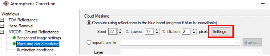
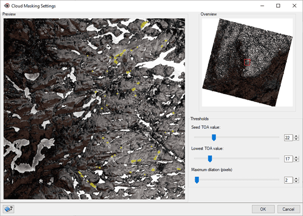
3.3. The Cloud Masking Settings widow will open. In this window you can adjust the Seed TOA, Lowest TOA and Maximum Dilation values. As you change these values you can see the changes that are made to the cloud masks in the Preview window. Experiment with different values to achieve the amount of cloud masking that you prefer. As you change the values make sure to pan around the image using the Overview window. You will notice in the preview image that clouds are masked but haze and water are not.
The following definitions from the help briefly outline each of the Threshold values.
3.4. Once you have the correct Threshold values click OK. The values will have populated in the ATCOR GUI.
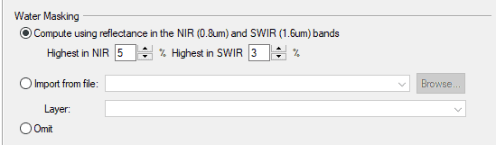
3.5. The following step allows you to specify the water masking options for your image. You can choose to create a new water mask, import a mask from file or omit the mask. The following values were set for the water mask.
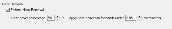
3.6. The final section in this step is to set the haze removal parameters. You can choose whether to perform haze removal or not. If you choose to perform haze removal you will need to enter the percentage of the image that is covered in haze and the maximum wavelength of the band on which to apply haze removal. The defaults of 50% and 0.85 micrometers were kept for this tutorial.
3.7. Click Next
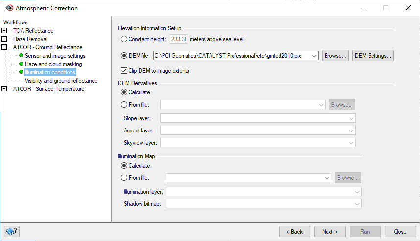
In the next window you can define the Elevation Information Setup by specifying a Constant Height value or by selecting a digital elevation model (DEM).
4.1. Define the Elevation Information Setup by specifying a Constant Height value or by selecting a digital elevation model (DEM).
If you do not have a DEM file, you can accept the default Constant Height which is a value that represents a constant elevation for the area covered by the image. This value is automatically populated using the gmted2010.pix file and the image center.
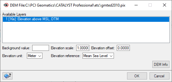
Otherwise, select the DEM File option and click the down arrow beside the field to select a DEM file available in the current session, or click Browse to select a file. When you select a DEM file, the DEM File window automatically appears listing the information for the selected DEM. This is automatically populated using the file’s metadata. The selected file must be reprojectable.
You may also click the DEM Settings... button to access this window.
4.2. If required for your data, specify options in the DEM Derivatives section to derive slope, aspect, and sky view information.
4.3. If required for your data, specify options in the Illumination Map section to calculate the illumination and shadow information.
4.4. Click Next
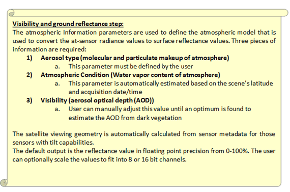
The visibility and ground reflectance options window is loaded. This section includes the Spectral Plot Tool. This tool allows users to experiment with different atmospheric settings to determine how they affect the reflectance values in the data.
5.1. Leave the Atmospheric Information and Satellite Viewing Geometry options as their defaults.
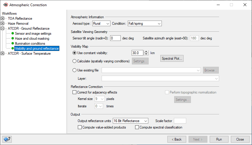
5.2. Under the Visibility Map section select Calculate (spatially varying conditions). By default, the ATCOR workflows uses a constant visibility of 30 km. You can set the constant visibility to a different value up to 180km. Alternatively, you may also calculate a visibility map for varying atmospheric conditions if the red and NIR bands are provided.
5.3. Click Settings. This will calculate a visibility map for varying conditions. The program will compute a visibility map for the scene, using Dark Vegetation pixels. These are defined based on NDVI and top-of-the-atmosphere reflectance in the red band.
5.4. Click OK

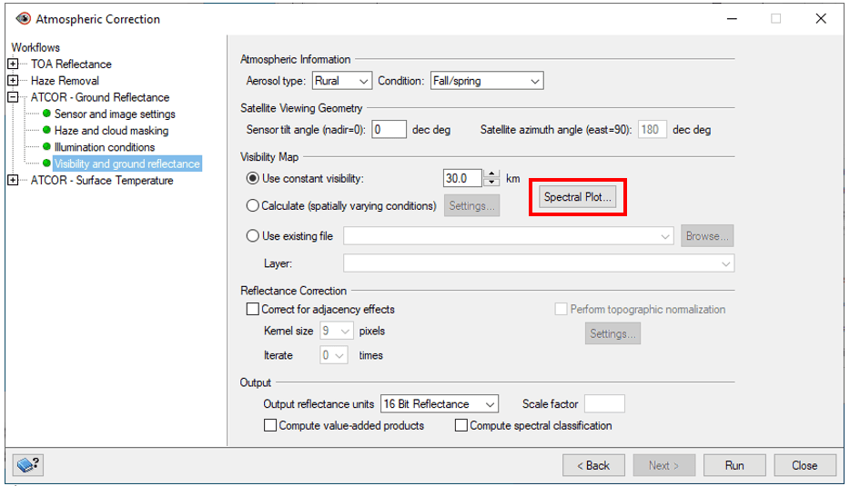
5.5. The option to choose an existing file that contains the visibility values is available by selecting Use existing file. The specified file must be reprojectable to the image, and the image must be fully contained within the visibility map. Once visibility has been determined you can click on Spectral Plot…
With this tool, users add library signatures to the graph and compare the reflectance values of their image to the library spectra. The graph will adjust the image reflectance values based on the placement of the crosshair pointer on your image. You can compare analogous ground cover types in the image to their corresponding library spectra. For example, the user can compare a pixel of a pine tree in an image to the library signature for pine trees and test different atmospheric settings to get the closest match. This provides confidence to the user that the atmospheric settings accurately model the atmosphere at the time of the image capture.
In addition to imagery, a spectral library is also required for use with the spectral plot tool. Spectral libraries are available from the ATCOR folder (C:\PCI Geomatics\CATALYST Professional\atcor\spec_lib).
6.1. If not already loaded, select Spectral Plot...
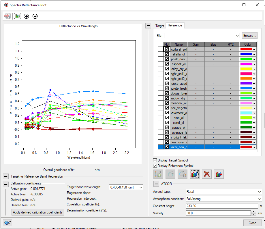
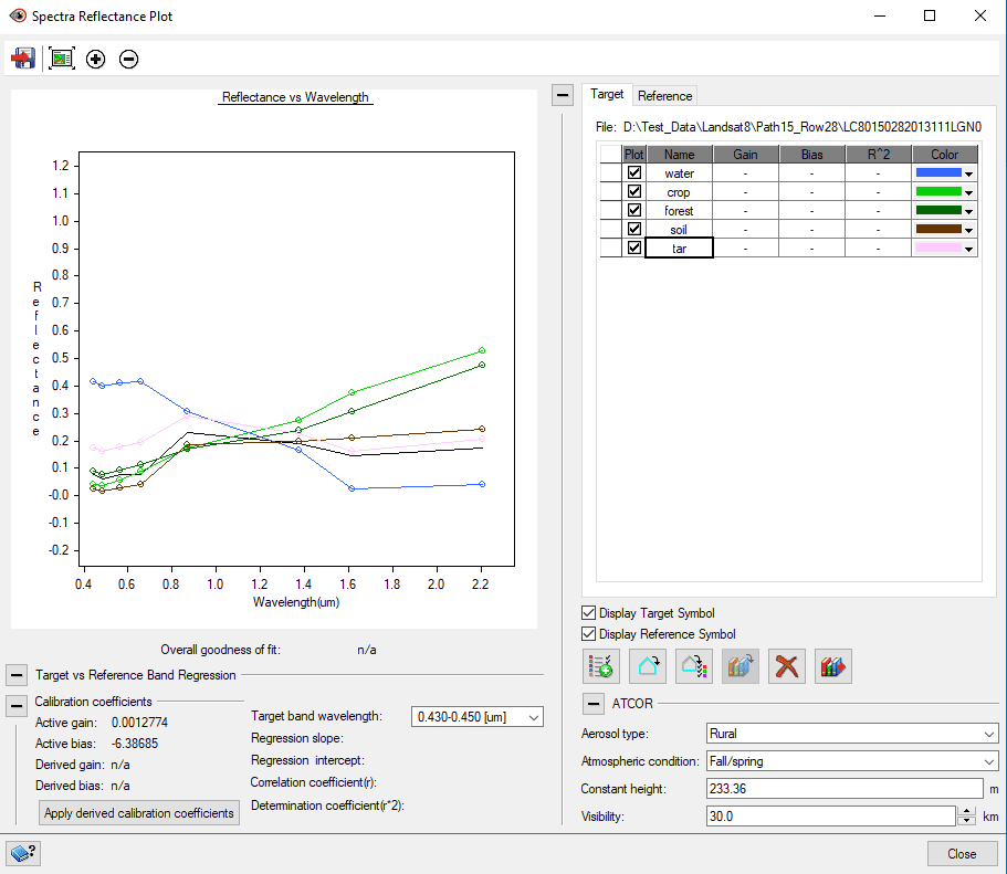
6.2. The Spectral Reflectance Plot window opens and the multispectral image is loaded into the Focus window. The main purpose of this window is to determine how similar your atmospherically corrected values are to library spectra. In the Spectral Plotting window you will see a Target and Reference tab.
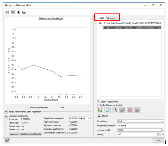
6.3. Click on the Reference tab
6.4. Click the Import spectra icon. The Open Reference Spectra window loads and the corresponding sensor spectral library are automatically populated.

6.5. Shift and select all of the reference spectra available.
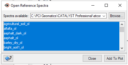
6.6. Click Add To Plot
6.7. Uncheck all of the classes so they are no longer visible in the plot window. We will come back to these later.
6.8. Click on the Target tab
6.9. Click the New Spectra icon five times. This will add five new classes to the Target window.

7.0 Click on the name of the class and modify it to your required new class name
7.1 Click on the arrow besides the Color field and modify the color for each class
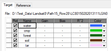
7.1. Select the water class from the Target window
7.2. In the Focus viewer you will notice a new layer has been added under the New Area Maps tab. Select this layer: New target layer.
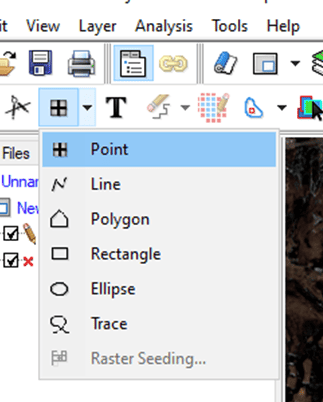
7.3. Select the New Shapes icon on the Focus toolbar and select Point. When collecting data for each class it is required that you collect point data and try to collect information in a linear fashion.
7.4. Select an area in the middle of a large water body and click to drop a point. Drop a number of points to collect more information. You will notice the graph shown in the Spectra Reflectance Plot changes based on the new information provided.
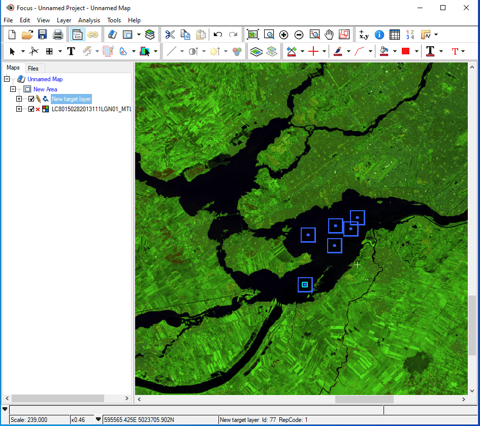
7.5. You can change the order of your bands in order to better see certain classes. In this case I’ve modified my image to show band order R:5 G:6 G:2 which better shows healthy vegetation. To change the band order, right click on the image in the Maps tab and select RGB Mapper. Modify the channels as required.
7.6. Select the next class in the Spectra Reflectance Plot list: crop
7.7. Select the new shapes point tool and collect points representing the crop class
7.8. Repeat the steps above to collect samples for the remaining classes
7.9. Once complete you will see all of the collected classes represented in the graph
8.1. In the Target tab select the water class to view. Uncheck all other classes.
8.2. Select the Reference tab
8.3. Compare all of the water specific signatures to your data. You will notice that the water_bright_lake_ol signature is the best match to the collected data.
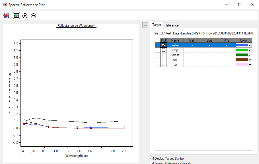
The example shows that the colored lines represent the library spectra. The black line represents the pixel that the curser is currently placed on in the Focus viewer and the blue line represents the collected data for our class.
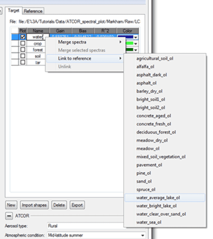
8.4. On the Target tab, right click on water and select Link to Reference > water_bright_lake_ol
8.5. You will notice the Selected Spectra goodness of fit for this link is 0.965. Ideally we would want a correlation coefficient closest to 1. If you notice that your correlation coefficient for water is not high, this is expected as water does not normally give off the best results due to its very low signal.

8.6. Continue to link the rest of the classes with the best matched reference signatures.
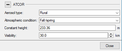
8.7. To improve the goodness of fit value, we will adjust the ATCOR parameters. In the ATCOR section of the Spectral Reflectance Plot panel you can modify the Aerosol type, Atmospheric Conditions, Constant height and Visibility.
We will select all of the classes that we want to keep in the analysis. Skip any class that had a poor correlation coefficient to exclude them from the calculation. Ctrl and Select all of the classes to include. The selected classes will appear in blue.
8.8. Under the ATCOR section of the window, update the Aerosol type, Atmospheric condition, Constant height and Visibility for your image. Notice the Selected Spectra goodness of fit value changes based on your input.
Experiment with the atmospheric information to see which information best matches your data. If these were set as constant values you can experiment with the values to determine how changing them will affect the Spectral Reflectance Plot.
8.9. Once you are satisfied with the variables from the Spectral Plotting window click Close. The values that you changed in this window will be modified and saved in the ATCOR window.
You can now run the atmospheric correction.
9.1. At the bottom of the ATCOR window click Run.
When the operation is complete, a new ATCORCorrected layer appears in the Focus Tree List, along with the generated masks, visibility map, terrain, and illumination files.
The atmospherically corrected image can now be used in further analysis. You will notice that the cloud mask is identical to the mask that you defined in the cloud masking tool. The masks can be used in future workflows to exclude these areas of the image from the analysis.
The illumination map helps to normalize affects caused by solar illumination. The map helps the algorithm determine how illuminated a pixel is regardless of the surface feature type. This is based off of the solar angle, relative to the slope and aspect angle of the pixel. For example, pixels oriented towards the sun are brighter, whereas pixels oriented away from the sun will be darker in the map.
The information set in the workflow tasks (Sensor and image settings, Haze and cloud masking, Illumination conditions, and Visibility and ground reflectance) is shared with all other Atmospheric Correction workflows, allowing you to reuse the same information to perform other tasks without having to re-specify the settings. Note, however, that all workflows apply to the same data set; specifying a new input data set in another workflow will overwrite the existing information.
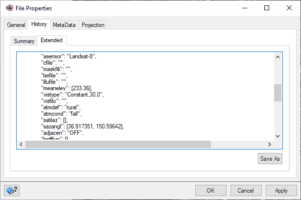
An after product of the ATCOR images is the log file recorded to the files History. These log files tell you the parameters which were used during atmospheric correction and can be used for future image processing or as metadata.
10.1. To view the parameters used in the ATCOR workflow, click on the Files tab
10.2. Expand the ATCOR corrected image
10.3. Right click on the image and select Properties
10.4. The File Properties window opens. Click on the History tab then click on the Extended tab.