Parameter descriptions
MFILE
The data to mosaic.
Input images can vary in projection, spatial resolution, or both. When the projection varies, the default output projection will be that which occurs most commonly in the input imagery.
You can specify the value of the parameter by using any of the following options:
- A specific data-file name or folder path and file name; for example, irvine.pix or C:\data\irvine.pix.
- A specific file-name pattern or all of the files in a folder; for example, C:\data\*.pix or c:\data.
- A text file that contains references to multiple files with, optionally, different parameter settings per file; for example, C:\list.txt or C:\list.mfile.
- The file, containing multiple files and different parameter values, must have a .txt or .mfile file name extension.
- List each set of parameters on its own line in the given order.
- Specify string parameters in quotation marks.
- Do not specify numeric parameters in quotation marks.
- A quotation mark preceded by a backslash is used as part of the string; for example, 'ab\"c' is used as: ab"c.
- Use an exclamation mark (!) before writing a comment in the text file.
- Use semicolons to delimit the parameters.
- When you do not want to specify a value, leave the position between the semicolons empty (";;"). Alternatively, if there are no remaining parameters to be specified at the end of a line, you can leave it blank.
- Parameters in a text file may or may not be specified in the algorithm:
- When a parameter is specified in the algorithm and in the text file, the value provided in the text file is used.
- When a parameter is not specified in the text file, you can do so in the algorithm.
-
Each line in the text file must follow this format:
<FILE>; [<NODATVAL>]
For example, C:\Data\image.pix; 0 indicates that a zero will be used as the background for the image.pix file.
You can also specify more than one NoData value. For example, C:\Data\image.pix; -32768, 0 indicates that -32768 will be used as the background for the first channel of the image.pix file, and zero (0) will be used for the second channel. You can, if necessary, skip a channel when specifying NoData so that all pixels in the channel are valid. For example, if you want to mosaic three images, each with different rules for NoData, specify your entry in the MFILE text file as follows:"c:\data\image1.pix"; -9999 ! all channels use -9999 as their NoData "c:\data\image2.pix"; 0, -9999 ! channel 1 uses 0 for its NoData and the remaining channels use -9999 "c:\data\image3.pix"; ,0,-9999 ! channel 1 does not have a NoData (notice the comma before the zero), channel 2 uses 0 for its NoData and the remaining channels use -9999
SILFILE
The name of the mosaic project file (.mos) to create.
An accompanying folder, with the same base name, is also created. The folder contains auxiliary information that makes up the mosaic project created by the mosaic-preparation process. Unique image IDs are created automatically based on the names of the source files and listed in the project file.
You can open the output mosaic project in CATALYST Professional Mosaic Tool to enhance the mosaic and perform quality-control procedures.
NODATVAL
The background value of the input images.
A pixel you designate as NoData is excluded from normalization, color balancing, and cutline generation. Images often have NoData defined in their metadata so this parameter can be defaulted.
When you specify a text file as input, you can specify the NoData value of an image in the file. The NoData value specified in the input text file takes precedence over all other sources. When a value is not specified in the text file, precedence is applied to the NO_DATA_VALUE metadata tag of the input image. If NO_DATA_VALUE metadata exists for an input channel, its value is used; otherwise, the NO_DATA_VALUE at the file level is used. Finally, if a NoData value is available in neither the text file nor the metadata, you can specify the value for this parameter.
- Text file
- Channel metadata
- File metadata
- NoData parameter value
If necessary, you can enter more than one NoData value for your input images. For example, to specify that channel 1 has a NoData value of -9999, channel 2 is 0, and channel 3 is 255, enter -9999,0,255.
SORTMTHD
The order in which to mosaic the images.
- NONE: Source images are processed in the order in the text file specified for MFILE. The first image in the file is the first processed. When the value of MFILE includes a wildcard or is a folder, the images are processed in ascending alphabetical order.
- NEARESTCENTER, [<starting_image>]: When you specify a starting_image, it is processed first; otherwise, the image most central of the input scenes is processed first. Subsequent images are processed based on which image has its center closest to the center of the first image. The center point is determined based on the rectangular bounding box of each image.
- MAXINTERSECT, [<starting_image>]: When you specify a starting_image, it is processed first; otherwise, the image most central of the input scenes is processed first. Subsequent images are processed in turn, based on which image most intersects (overlaps or covers) the images processed already. Each calculation, such as determining overlap amounts, is based on the rectangular bounding box of each image.
This parameter is optional.
NORMALIZ
The normalization to apply to each source image before color balancing, cutline generation, or mosaicking.
Occasionally, images can contain patterns in visual brightness that affect the seamless integration of the images into a mosaic. By applying normalization, bright and dark effects in images are evened out to create a mosaic that is more pleasing visually.
Each normalization method applied (except NONE) results in some coefficients that define a transformation of pixel values in the source image. These are written to the source-image description file.
- NONE: No adjustment of the pixel values of the source images occurs.
-
HOTSPOT: Removes hot spots from the input images.
A hot spot is a common distortion in aerial photographs and optical-satellite images. With aerial photographs, distortion is caused typically by solar reflections that appear circular (also known as lens flare). With optical-satellite images, distortion appears typically as a striped pattern.
HOTSPOT normalizes the brightness over the image by fitting a Gaussian surface to the brightness values. Smaller spot reflections, such as from lakes, cars, or buildings are not removed.
-
ADAPTIVE, [<image_percent>]: Balances the brightness and contrast by using a moving window. The method is well suited for use on images with a large, irregular bright-and-dark pattern that cannot be modeled to a Gaussian surface. Patterns that model to a Gaussian surface are better processed with HOTSPOT.
ADAPTIVE adjusts the brightness and contrast over local areas, improving image detail, while reducing the bright-and-dark pattern over the entire image. The method applies an adaptive enhancement by using a moving window to calculate the adjustment for each pixel value.
The size of the window affects the results of the filter. You specify the window size by entering the percentage value of the filter size; for example, to represent a 35-percent window, enter 35. If you do not specify a value for image_percent, a default value of 20, or 20 percent, is applied.
ADAPTIVE calculates the mean and standard deviation of the gray levels in the window and adjusts the values to match the overall mean and standard deviation of the image. Mean adjusts the brightness and standard deviation adjusts the contrast.
This parameter is optional.
BALSPEC
The color-balancing method to apply.
Color balancing evens out the color contrasts between images to reduce the visibility of seams and produce a mosaic that is appealing visually. Each method (except NONE) results in some parameters that define an adjustment of pixel values in the source image. The adjustments are applied when the image is added to the mosaic and stored as part of the mosaic project.
-
BUNDLE, [AUTOSCALE], [DODGE=MANY, [SAMPLE=<size>], [DIST=<distance>]]: Produces best-looking color-balancing results by using two complimentary phases.
First, a global adjustment of the mean and sigma of each image is computed by using a "block-bundle" method between it and each of its overlapping images. The method makes large adjustments between images to make them more balanced.
Second, a series of dodging points is determined automatically to make smaller local adjustments between pairs of images. The order of the input images is ignored, because all of the overlapping images are used to adjust one image.
You can also specify the keyword AUTOSCALE to have all input images stretched linearly and have a common scale. This can improve the results when the dynamic ranges of various input images vary significantly. You can also specify the keyword DODGE=MANY to allow the creation of multiple dodging points for each edges across the whole project, rather than just one dodging point per edge. When DODGE=MANY is specified, you can also use the SAMPLE=<size> and DIST=<distance> keywords to further control the dodging points. To adjust the number of full-resolution pixels that are used to compute each dodging point specify a value for the sample <size>. To adjust the spacing between the dodging points specify a <distance> in the units of the project. When unspecified, a default <size> of 64x64 is used, while a <distance> is computed automatically. For example, BALSPEC="BUNDLE, DODGE=MANY, SAMPLE=128, DIST=1000" would result in dodging points being created every 1000 meters, with each point using the surrounding 128x128 pixels. -
OVERLAP: Bases color balancing on matching overlapped areas of the input images.
The rasters must have a sufficient overlap (greater than 10 percent) between each pair of adjacent input rasters and have good-quality georeferencing. You can also specify a local (LOCLMASK) or global mask (GLOBMASK). The mask must have some pixels within the overlap area to affect the output.
-
LUT, <LUT_segment_number>: Color balancing is determined by lookup table (LUT) segments stored previously from the source images.
When you specify a LUT value, MOSPREP looks for one LUT segment for each image channel; for example, an RGB-color image being added to the mosaic must have three LUT segments per input file.
LUT-segment numbers must be provided explicitly using LUT_segment_numbers. The first LUT is used for the first image channel, the second LUT for the second channel, and so on. All input images must have the specified LUT segments; otherwise, the process will stop and an error message is displayed.
-
HISTOGRAM, [<match_area_multiple>], [<trim_percentage>]: Color balancing is based on matching the histogram of the input image to that of the target mosaic image, sequentially.
The match_area_multiple value determines the amount of data in the mosaic file to use to compute the reference histogram.- When you specify a value of 1, the reference histogram is computed based on an area equal to the overlap between the incoming image and the output mosaic.
- When you specify a value of 3, the reference histogram is computed based on an area equal to three times the overlap between the incoming image and the output mosaic.
-
REFERENCE, <fili_ref>: Color balancing is based on matching source-image histograms with those of the specified reference image.
The reference-image file is specified by fili_ref. The reference image need not be the same resolution or projection as the input images, provided it can be reprojected into the projection of the input image. That is, neither precise georeferencing nor overlap are required.
-
NEIGHBORHOOD, [<meanb_adjustment>], [<outlier_correction>], [<outlier_threshold>]: Determines a set of model coefficients that change each image pixel based on the pixel values of the intersecting (neighboring) pixels, regardless of image order.
The overall pixel value of each individual image is adjusted iteratively, such that the value is similar to those of its neighboring images.
- meanb_adjustment, set to 3 by default, adjusts the overall tonal value of the image pixels in each overlapping region to minimize the outliers.
- outlier_correction excludes extreme pixel values–outliers–from the computation of the coefficients. The default is YES.
- outlier_threshold is for use only when the value of outlier_correction is YES. The default value is 1, which excludes from the computation of the coefficients pixel values beyond the mean difference value, plus one standard deviation.
When you specify NEIGHBORHOOD, MOSPREP uses the default values of meanb_adjustment, outlier_correction, and outlier_threshold.
- NONE: Images are added to the mosaic as is and the pixel values are not adjusted
This parameter is optional.
LOCLMASK
Whether to apply a local mask to exclude specific pixels from color balancing or from cutline generation.
You use a mask when the same feature or features differ radically from one image to another.
LOCLMASK = (NONE | BIT | VEC | <n>), (NONE | BIT | VEC | <n>)
The first parameter value refers to color balancing and the second refers to cutline generation. Regions specified with the second parameter are used as local constraints during cutline generation.
- NONE: Do not exclude any pixels from the computation.
- BIT: Use when at least some of the source images have bitmap segments that define exclusion regions. When one of the source images contains multiple bitmaps, the last one is used. All image pixels covered by the bitmap are excluded from calculation.
- VEC: Use when at least some of the source images have vector segments that define exclusion regions. When one of the source images contains multiple vector segments, the last one is used. This vector segment must be a polygon, and all image pixels enclosed by the polygon are excluded from the calculation.
- <n>: Use the bitmap or vector segment of the specified number, <n>, as the mask.
Note: If two segments share the same number, MOSPREP uses a bitmap segment over a vector segment to define the mask area.
- BIT, BIT: Uses the last-created bitmap for both color balancing and cutline generation.
- NONE, VEC: Uses all data for color balancing, but excludes data under polygons in the last-created vector segment from cutline generation.
- VEC, 3: Uses the last-created vector segment for color balancing, and uses segment 3 as a local cutline constraint.
- 4: Uses segment 4 to limit color balancing, but does not constrain cutlines.
This parameter is optional.
GLOBFILE
The file that, in conjunction with the value of GLOBMASK, you can use to define a global exclusion mask.
A global exclusion mask identifies regions in the source images to exclude from color balancing or cutline generation. GLOBFILE provides the file name referenced by GLOBMASK.
GLOBFILE = (<cb_file> | NONE), (<cut_file>)
- <cb_file>: Path and file name of the mask file to use for global color balancing
- <cut_file>: Path and file name of the mask file to use for global cutline-avoidance areas
- NONE: Keyword used to specify no color balancing, but you can specify a cutline file; for example, NONE, <cut_file>
This parameter is optional.
GLOBMASK
In conjunction with the value of GLOBFILE, the global exclusion mask that identifies regions in the source images to exclude from color balancing or cutline generation.
Typically, you use the global exclusion mask to identify large areas to exclude from color balancing, such as a large body of water. The mask can also include building footprints to influence the cutlines that MOSPREP generates. However, because the specified mask assigns a high cost to masked regions, cutlines will generally avoid such regions unless there is no better alternative.
You can specify a bitmap or a vector as an exclusion mask, both of which refer to the file specified for GLOBFILE. If you do not specify a value for this parameter, no mask is applied.
GLOBMASK = (-1 | <n>), (m)
- <n>: Defines the segment number that corresponds to the color-balancing mask (cb_file) in the file specified for GLOBMASK. This value must be specified as -1 if–and only if–no color balancing is defined (GLOBFILE = NONE).
- <m>: Defines the segment number that corresponds to the cutline-avoidance mask (cut_file) in the file specified by GLOBMASK.
This parameter is optional.
CUTMTHD
The method to use to generate cutlines (polygons that enclose all of the data) from an image to include in the output mosaic.
You can specify the value as follows:
CUTMTHD = <method>, [(<vector_file>, [<field_name>], [<segment_number>]) | (AUTOCONSTRAIN[=CLASSIC[,<thiessen_factor>]] | [=STRIPS[,<overlap_factor>]]), [VECTHIN=<thin_tolerance>], [DOWNRES=<x_resolution>[;<y_resolution>]], [ERODEEXT[=<erosion_distance>]], [FORCE_DATAEXT]]
The keyword identifying the method is mandatory, but you can, optionally, specify other settings to further influence the cutlines. In particular, you can specify options related to constraining polygons, which define regions in which cutlines are allowed for each image, such that the generated cutlines do not cross the specified boundaries or thinning the cutlines, which reduces the number of vertices.
- Specify an existing cutline-constraint file
- Automatically generate a cutline-constraint file using the classic method which is based on the center of each image
- Automatically generate a cutline-constraint file using a "strips" method which is based on the overlap between images
Specify a cutline constraint file
- Name of the vector (vector_file)
- Name of the attribute field that contains the image source (field_name)
- Number of the vector segment that contains the constraint polygon (segment_number)
- the value of its file level metadata tag: SourceID, or if that tag does not exist, then
- the base name, without the extension, of the input source image's file name.
If the field_name is not specified, MOSPREP searches the vector-segment attributes for a field named ImageSource. If the specified field name or ImageSource does not exist, an error occurs.
If the segment number is not specified, the algorithm uses the last segment from the vector file you specified. If the constraining polygon is larger than the image being processed, cutline generation is not constrained. If the constraining polygon does not overlap the image, an error occurs.
Automatically generate a cutline-constraint file
You can use the AUTOCONSTRAIN option to automatically generate a constraining polygon layer. By doing so, MOSPREP will generate one constraint polygon for each input image. If the input images are approximately square and contain a lot of overlap, the classic constraint polygons limit the data to consider for cutline generation to only the central parts of each image. Alternatively, if the images have one side much longer than the other than the strips method is likely better for constraining the cutline generation.
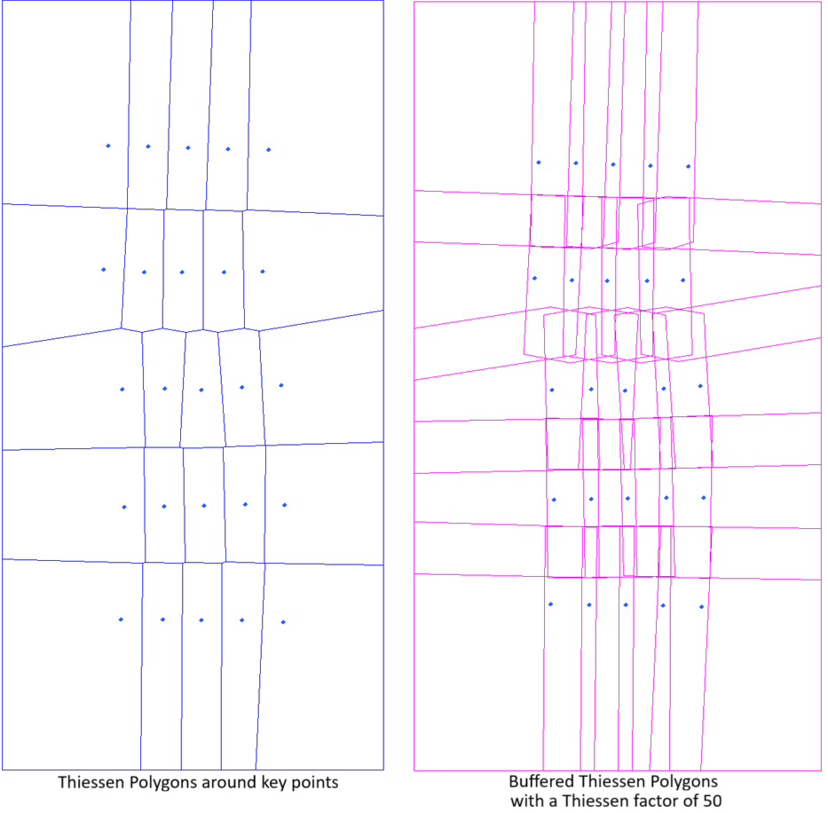
The AUTOCONSTRAIN=CLASSIC option is ideal for use with airphoto projects, because, such projects have typically a large amount of image overlap. You can adjust the option by specifying a Thiessen factor (thiessen_factor). The value you specify can range from 1 through 100. A larger value causes more overlap between the generated constraint polygons; that is, the cutlines will be less constrained. If you do not specify a value, the default value of 50 is applied. If AUTOCONSTRAIN is specified without a further keyword, it is interpreted as if CLASSIC were provided so AUTOCONSTRAIN=40 is treated as AUTOCONSTRAIN=CLASSIC,40.
The AUTOCONSTRAIN=STRIPS option is best suited for projects that have a clear pattern of strips, such as often seen with ADS data. Images must be of similar size and align in at least one direction from, for instance, aerial flight lines or satellite swaths. Cutline-constraining polygons will be generated for each image based on where it and its neighbors have actual data. This method first tries to group the images in rows or columns, and will choose the strips with the most consistent distance between images. It will then remove the overlap between images in each strip using, at most, two neighboring images. Finally overlap will be remove between the different strips leaving a constraining polygon. The extents of the polygons can be manipulated by specifying a value between 1 through 100 for the overlap factor (overlap_factor). A larger value causes more overlap between the generated constraint polygons; that is, the cutlines will be less constrained. If you do not specify a value, the default value of 30 is applied.
The VECTHIN option controls the thinning, or weeding, of the computed cutlines. When you want the cutlines, with all of the vertices computed initially, included in the output, enter a thin-tolerance value of 0. Any number greater than zero increases the thinning of the vector, so the cutlines will have fewer vertices. Approximately, a value of n results in 1/n of the vertices being written to the output. When you do not specify a value, a default value of 1.75 is applied (VECTHIN=1.75).
The DOWNRES option controls the resolution of the mosaic preview. It can be used to override the default reduced-resolution used by the algorithm. The applicable units are those of the projection of your project. For example, to use a 8 meters resolution of an UTM project, enter CUTMTHD="MINSQDIFF, DOWNRES=8".
- MINSQDIFF, [(<vector_file>, [<field_name>], [<segment_number>]) | (AUTOCONSTRAIN[=CLASSIC[,<thiessen_factor>]] | [=STRIPS[,<overlap_factor>]]), [VECTHIN=<thin_tolerance>]]: The minimum squared difference method. Well suited to to most mosaicking projects, this method, in most cases, produces the cleanest cutlines. The algorithm determines a cutline in each overlapped area between two adjacent images, with minimum squared differences of gray values at the same locations of the region in all image channels.
- MINDIFF, [(<vector_file>, [<field_name>], [<segment_number>]) | (AUTOCONSTRAIN[=CLASSIC[,<thiessen_factor>]] | [=STRIPS[,<overlap_factor>]]), [VECTHIN=<thin_tolerance>]]: The minimum difference method. With this method, the algorithm determines a cutline in each overlapped area between two adjacent images, with minimum differences of gray values at the same locations of the region.
- MINRELDIFF, [(<vector_file>, [<field_name>], [<segment_number>]) | (AUTOCONSTRAIN[=CLASSIC[,<thiessen_factor>]] | [=STRIPS[,<overlap_factor>]]), [VECTHIN=<thin_tolerance>]]: The minimum relative difference method. Similar to MINDIFF, this method provides better output when similar sections of data appear dissimilar in various images.
- EDGE, [(<vector_file>, [<field_name>], [<segment_number>]) | (AUTOCONSTRAIN[=CLASSIC[,<thiessen_factor>]] | [=STRIPS[,<overlap_factor>]]), [VECTHIN=<thin_tolerance>]]: The edge-feature method. This method provides better output in urban-area mosaicking or in images containing many linear features. The objective of the EDGE method is to avoid placing cutlines across linear features.
- MAXDATA, [(<vector_file>, [<field_name>], [<segment_number>]) | (AUTOCONSTRAIN[=CLASSIC[,<thiessen_factor>]] | [=STRIPS[,<overlap_factor>]]), [VECTHIN=<thin_tolerance>]]: The cutlines to be on the boundary of the real image pixels, meaning that NoData pixels are ignored when the image boundary is determined.
- IMPORT, <vector_file>, [<field_name>], [<segment_number>]: Uses the specified polygons as cutlines, exactly as they appear in the vector file.
- FILEEXT: The cutline to be the extents of the input image or images and will not exclude NoData pixels from cutline generation.
Eroding the data-extents polygons
- ERODEEXT: shrinks each of the data-extents polygons by an amount determined automatically using the resolution of the mosaic preview. The polygons are buffered by the determined amount and retain only the area of the original polygon that is inside of the buffer boundary.
- ERODEEXT=<erosion_distance>: is similar to ERODEEXT, except uses the buffer distance specified via <erosion_distance>. The applicable units are those of the projection of your project. For example, to shrink the data-extents polygons of UTM data by 5 meters, enter CUTMTHD="MINSQDIFF, ERODEEXT=5".
By default, if an image does not overlap the current mosaic preview, it will be assigned a cutline equal to that file's extents. Consider using the keyword FORCE_DATAEXT if you prefer such an image to have its cutline be the image's data-extents. By doing so, you ensure MOSPREP creates data-extents polygons for each input image and that the cutline will be set to the image's data-extents if it does not overlap with the current mosaic preview. For example, the first image is, by default, assigned a file extents cutline because the mosaic preview is empty at the start.
When one image completely overlaps another in the same mosaic project, the computation of the cutlines differs slightly. Perpendicular profiles are drawn at intervals around the image boundary. For each profile, the location that gives the best result for your cutline criterion (for example, MINDIFF, MINRELDIFF, and so on) is selected as a "seed point". A dynamic programming algorithm is then used to find the minimum-cost path. This produces a cutline that can be merged to form a closed loop. This may appear as a "patch", because there is no starting and ending point but, rather, a looped cutline.
This parameter is optional.
MAPUNITS
The projection string or units of the mosaic preview and other MOSPREP output data.
If you do not specify a value for this parameter, the projection that occurs most commonly in the input imagery is applied. If you specify a projection that differs from that of the input data, the data is reprojected. A projection string must fully identify the projection and Earth model you want, such as UTM 17 D000.
The standard definitions are as follows:
- UTM: Universal Transverse Mercator
- SPCS: State Plane Coordinate System
- LONG/LAT: Longitude and latitude
- METER: Image along-row and along-column meters
- FOOT: Image along-row and along-column feet
- PIXEL: Pixel and line
For a complete list of supported projections and Earth models, see Map projections. For information on the format of the map-units string, see Output units.