INSMODGOLD
Apply a modified Goldstein filter to enhance Interferometric fringes
Description
INSMODGOLD uses local Fast Fourier Transforms (FFT) to enhance fringes in an interferogram. Doing so may reduce the time required for subsequent phase unwrapping.
Parameters
| Name |
Type |
Caption |
Length |
Value range |
| FILI * |
String |
Database Input File Name |
1 - 192 |
|
| DBIC |
Integer |
Database Input Channel List |
0 - |
1 - |
| FFTSIZE * |
Integer |
FFT window size |
1 - |
8|16|32|64|128|256
Default: 64 |
| FILO * |
String |
Database Output File Name |
1 - 192 |
|
* Required parameter
Parameter descriptions
FILI
This parameter specifies the name of the input file containing the interferogram to filter.
DBIC
The input interferogram channel or channels to be filtered. The specified channels must contain 32-bit complex values with interferograms that have not been unwrapped. The default value (blank) is to apply the modified Goldstein filter to all channels.
FFTSIZE
This parameter defines the size of the FFT window. Applying larger window sizes will reduce the interferometric noise but may destroy phase continuity in areas with a high number of fringes.
This size of the spectral window must be a power of two. The default value is 64.
FILO
This parameter specifies the name of the output file. The output file will contain filtered interferograms written as 32 bit complex pairs in the order specified by the
DBIC parameter.
Details
INSMODGOLD is normally applied after the topographic phase correction (INSTOPO) or after the orbit adjustment (INDSADJUS) to enhance interferometric fringes and possibly speed up the following phase unwrapping (INSUNWRAP).
INSMODGOLD applies a sliding 3x3 spatial boxcar filter to prefilter the data prior to estimating the fringe frequency. The prefiltered spatial data is converted to the spectral domain using the FFT size defined by FFTSIZE. The frequency within the FFT window with the largest magnitude represents the local fringe rate. The frequency representing the local fringe rate is removed from the original spatial data leaving the local residual noise. The residual noise is converted to the spectral domain and the magnitude of the noise peak is determined. If the local data (within the processing window) is highly coherent, the magnitude of the noise peak will be close to zero. For less coherent areas the magnitude of the noise peak will be larger than zero, but still smaller than the previously removed frequency representing the local fringe rate. The power of the residual noise is increased by a factor of alpha where alpha is a combination of the mean value of the local coherence and magnitude of the noise peak. Local areas with high coherence will have alpha values near zero and will be weakly filtered while regions with lower coherence and/or significant residual noise will be strongly filtered. The filtered spectral noise component is converted back to the spatial domain and combined with the previously extracted local fringe rate to restore the original characteristics of the interferogram. A sliding triangular weighting is applied to enhance the fringes and preserve the magnitude and phase continuity of the original interferogram.
Examples
Apply the modified Goldstein filter using an FFT window size of 64 x 64 to a file containing a single interferogram.
EASI>FILI="c:/interferogram.pix"
EASI>DBIC=
EASI>FFTSIZE=64
EASI>FILO="goldstein_filtered_interferogram.pix"
EASI>run INSMODGOLD
Apply the modified Goldstein filter using an FFT window size of 32 x 32 to the indicated channels. In this example, the output will be written to channels 1,2
EASI>FILI="c:/interferogram.pix"
EASI>DBIC=2,4
EASI>FFTSIZE=32
EASI>FILO="goldstein_filtered_interferogram.pix"
EASI>run INSMODGOLD
Algorithm
The first step is to prefilter the input interferogram
S using a simple 3x3 boxcar filter. The prefiltered interferogram is given as:
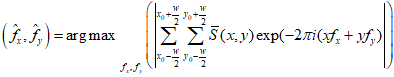
The prefiltered data is Fourier transformed to the spectral domain and the narrow band frequency with the highest magnitude which represents the local slope is extracted.
Where
w is the FFT window size and
fx
and
fy
represent the range and azimuth components of the local slope.
The slope compensated output
S'(x, y) in the spatial domain is given by:
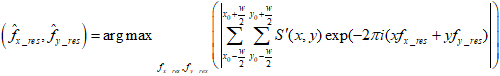
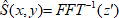
The slope compensated pixels are Fourier transformed to the spectral domain with
z = FFT(S') and in a similar manner as before, the maximum broadband frequency representing residual phase and noise is extracted and given by:
Where
fx_res
and
fy_res
represents the range and azimuth component of the residual noise.
We compute the modified Goldstein filter parameter
α by combining the mean of the local coherence

with the magnitude of the dominant residual component. The Goldstein filtered output is computed as
z' = |z|αz where:
Areas which are locally highly coherent will have
α values close to zero and are weakly filtered. Areas with high residual noise will have higher
α values and be strongly filtered. The Goldstein filtered residuals are returned to the spatial domain with
.
The local narrow band frequency  is combined with the modified Goldstein filtered residuals to give the final filtered phase value
  where
where  .
.
To preserve phase continuity, a final 2D triangular filter weighting is applied.
The algorithm is fully described in Feng et. Al.
References
Feng, Q., Xu, H., Wu, Z., You, Y., Liu, W., Ge, S. "Improved Goldstein Interferogram Filter Based Upon Local Fringe Frequency Estimation," Sensors 2016, 16, 1976.
Goldstein, R. M., Werner, C. L., "Radar Interferogram filtering for Geophysical Applications," Geophysical Research Letters, Vol. 25, NO 21. Pp 4035 - 4038, Nov. 1998.
© PCI Geomatics Enterprises, Inc.®,
2026. All rights reserved.