Details
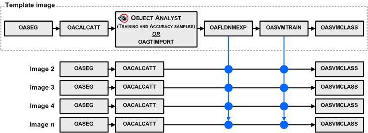
A typical workflow starts by running the OASEG algorithm, to segment your image into a series of object polygons. Next you would calculate a set of attributes (statistical, geometrical, textural, and so on) by running the OACALCATT algorithm. Alternatively, when you are working with SAR data, you would use OASEGSAR and OACALCATTSAR. You can then, in Focus Object Analyst, manually collect or import training samples for some land-cover or land-use classes; alternatively, use OAGTIMPORT for this task. The training samples are stored in a field of the segmentation attribute table with a default name of Training.
- A segmentation with a field containing training samples
- A list of attributes
You can create the list of attributes by running OAFLDNMEXP. Alternatively, the list can be read directly from the table of segmentation attributes using field metadata that was created by OACALCATT or OACALCATTSAR.
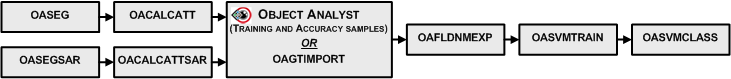
Typically, you specify as input the segmentation vector layer from OASEG or OASEGSAR.
The training (OASVMTRAIN) and classification (OASVMCLASS) steps are distinct to allow you to reuse a trained SVM model for other segmentations, provided that the list of attributes is the same for all segmentations and calculated from similar images; that is, from the same sensor and in the same acquisition mode.
SVM classification
Based on statistical-learning theory, Support Vector Machine (SVM) is a machine-learning methodology that is used for supervised classification of high-dimensional data. With SVM, the objective is to find the optimal separating hyperplane (decision surface, boundaries) by maximizing the margin between classes, which is achieved by analyzing the training samples located at the edge of the potential class.
These training cases are referred to as support vectors. The algorithm mostly discards (other) training sets beside the support vectors. This results in an optimal hyperplane fitting with effectively fewer training samples used. This implies that SVM achieves better classification results even with a smaller training set.
In its simplest form, SVM is a linear binary classifier. To use SVM for multiclass applications, two main approaches have been suggested, with the basic idea being to reduce multiclass to a set of binary problems.
The first approach, which is used by PCI technology, is called one against all. This approach generates n classifiers, where n is the number of classes. The output is the class that corresponds to the SVM with the largest margin. With multiclass, it must interpret n hyperplanes. This requires n quadratic programming (QP) optimization problems, each of which separates one class from the remaining classes.
The second approach, which is not used by PCI technology, is one against one. This approach combines several classifiers and can perform pair-wise comparisons between all n classes. Therefore, all possible two-class classifiers are evaluated from the training set of n classes, each classifier being trained on only two out of n classes, giving a total of n(n–1)/2 classifiers.
Applying each classifier to the test-data vectors gives one vote to the winning class. The data is assigned the label of the class with the most votes.
SVM kernels
When two classes are not discriminable linearly in a two-dimensional space, they might be separable in a higher-dimensional space (hyperplanes). The kernel is a mathematical function used by the SVM classifier to map the support vectors derived from the training data into the higher-dimensional space.
- Radial-basis function (RBF)
- Linear
- Polynomial
- Sigmoid
Typically, the RBF kernel provides the best results.
The polynomial kernel is fixed to the third order.
Optimization and cross-validation
Each SVM kernel has its own set of parameters that affects the behavior of the kernel. For example, each kernel includes a parameter constant (C) that penalizes the model when it gets over-fit.
A specific optimization procedure is used and, using the concept of cross-validation, the appropriate values for the parameters (C et al.) are calculated during model training. The calculated parameter values achieve generally the best accuracy for the training samples while reducing the possibility of model over-fitting.
Normalization of data
It is recommended to normalize data so that each attribute can be treated equally to discriminate classes. Normalization is particularly necessary when all attributes are mixed from various types; for example, the mixture of spectral values with geometrical ones, or various SAR parameters and texture features. Attributes are normalized by using linear scaling to produce a range from zero through one; that is, the minimum value is mapped to zero, the maximum is mapped to one, and the values in between are scaled linearly.
Output fields
In Object Analyst, during Training Sites Editing, you define a series of classes and collect training and accuracy samples.
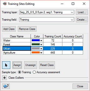
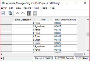
The Class field contains the class name of each object, as defined in Object Analyst during Training Sites Editing.
The Label field contains a label for each class and corresponds to an integer. The class number (label) is attributed during the SVM training. Each class label corresponds to a unique class number.
The Probability field contains the voting probability (class membership), distributed between zero and one, for each object. An object and its associated attributes can belong to more than one class, as defined by the classification hyperplanes. An object will belong to the class getting the most votes. The higher the voting probability, the stronger is the membership of an object to a single class.