Parameter descriptions
Input Scenes
The path and name of the folder containing the raw images to process.
- Path and name of a folder of input images; for example, C:\data.
- Path and name of a folder with a wildcard to filter the imagery by file name or type; for example, C:\data\*.xml.
- You can also specify an MFILE as input. An MFILE is a text file with an .mfile file name extension. For more information on this type of file, see About the MFILE format.
Output Folder
The path and name of the folder to which to write the output files.
If tiled output is specified, tiles are processed by the processing nodes configured by the CATALYST Enterprise, and are stored in the specified output folder. Local copies of the tiles on processing nodes are automatically deleted. The output tile file names are generated automatically according to the Tile Base Name.
Ingest Method
Select whether to link or import the data specified in the scene folder.
- Automatic: Links or imports the data based on the sensor.
- Import: Creates from the file in its raw vendor format a PCIDISK file that contains the input scene.
This method may take longer to ingest the data; however, it improves the overall performance of the workflow.
Important: The Import method requires twice the amount of disk space, because it duplicates the pixel data. - Link: Creates a PCIDISK file that points to the input scene.
This method ingests data very quickly; however, subsequent steps of the workflow may take longer to complete.
Output File Type
The format of the output file.
For more information on the supported file formats, see GDB-supported file formats.
Output File Options
The options to apply when creating the output file or files. The available options are specific to the file format; in each case, the default of no options is allowed.
For more information on the options available for the output file type you specify, see GDB-supported file formats.
Overwrite Results
Select this check box to overwrite the existing output files, if any exist. If this check box is left clear, and an output file exists in the relevant folder, the status of the job displays a message informing you of the existence and name of the output file. The message is also written to the event log of the job.
Send Email
If necessary, you can set up CATALYST Enterprise to send an email notification on job start and job completion.
With this check box selected, an email message is sent to each address specified in the Email Addresses box after the job starts and on completion.
You can specify one or more addresses, and each must be separated by a comma or a semi-colon. The email address of the user currently logged in displays by default.
Product Type
From the list, select the type of product you want to mosaic.
- Multispectral (MS)
- Panchromatic (PAN)
- Pansharpened (PSH)
- MS & PAN (for Pansharpening)
This parameter is optional.
Math Model Filter
The math model to use for collection of ground control points (GCPs) and, subsequently, orthorectification.
- Automatic: available in data-ingest-related modules only, such as the Data Ingest and GCP Collection module. With this option selected, any and all supported math models is added to the output file for each scene. Typically, only the selected math model is added to the output files.
- Rational Function Model (RPC): uses the Rational Polynomial Coefficients (RPCs) that are distributed with the raw imagery. With most modern sensors, this is the most robust model to use, as the distributed RPCs are very well calibrated (accurate). Therefore, fewer GCPs are required, generally, and positional improvements are not constrained to areas within the outer bounds of the GCPs collected. Other abbreviations for the Rational Function Model include RF, RFMODEL, RFI, RF0, RF1, and RF2.
- Toutin's Satellite Orbital Model (Rigorous): CATALYST Enterprise uses the Toutin rigorous math-model solution, which calculates the position and orientation of the sensor at the time of image capture from an orbital or ephemeris segment. When this information has been identified, it can then be used to accurately account for known distortions in the image. After the sensor orientation and position have been calculated, this information can be used to drive other processes, such as orthorectification. Other abbreviations for Toutin's Satellite Orbital Model include SAT, RIG, SRIT, and TOUTIN.
The module first attempts to use the selected math model. If required information is missing from the user-defined math model, the module automatically tries to use another math-model option, and displays a warning message.
RF Math Model Order
When using the Rational Function with satellite imagery, you can modify the RF math model to better agree with collected ground control points (GCPs) by selecting the correct RF math-model order.
- Order 0: allows x,y translations
- Order 1: allows x,y translations with rotation
- Order 2: allows x,y translations with rotation and increased warping
Typically, performing a first-order transformation is best, except when the GCPs are not well distributed. If your GCPs are clustered together, a first-order transformation may introduce new and significant errors in the image away from the GCPs. If your GCPs are not well distributed, you will probably obtain better results with the zero-order transformation.
Source Background Type
The method to use to determine which pixels in the source image to process as background (NoData) pixels. In general, if a pixel is considered NoData, the module processes it in a specific manner.
If the Any option or the All option is selected, a value must be specified for the Source Background Value parameter.
-
File Metadata, else None: reads the NoData value from the input-file metadata. The module first checks for the file-level metadata tag NO_DATA_VALUE in the source raster. If the tag is present, this value is used as a default for all channels in the file. Next, the module checks for channel-level NoData tags; if one is found, the channel-level value overrides the file-level value for that channel.
If there are channel-level NoData tags, but no file-level tag, a pixel is considered as NoData if each of the channels with a NoData tag corresponds to its NoData value. In this case, channels without a NoData tag are ignored when identifying background pixels.
If the file does not contain NoData tags, all pixels in the source image are considered valid.
- None: all pixels in the source image are to be considered valid
- All: if the pixel value in all channels matches the values provided for the Source Background Value parameter, the pixel is considered background (NoData).
- Any: if the pixel value in any channel matches the value provided for the Source Background Value parameter, the pixel is considered background (NoData).
For specific examples, see the Source Background Value parameter description.
Source Background Value
- All
- Any
The source background value is provided as either a single number (applied to all channels) or as a pixel "stack" (a comma-delimited list of values). If a pixel stack is provided, but the number of values does not equal the number of channels, the list is truncated or the last value is repeated as necessary. The background values provided is truncated to the range allowed by the source image data type.
-
Source Background Type set to All and Source Background Value set to 0: a pixel is considered background if all three channels are zero.
- Source Background Type set to Any and Source Background Value set to 0: a pixel is considered background if any of the three channels is zero
- Source Background Type set to All and Source Background Value set to 128,0,0: a pixel is considered background if its value is exactly 128 for the first channel and zero for the second and third channels
- Source Background Type set to All and Source Background Value set to 128,0,0,245: a pixel is considered background if its value is exactly 128 for the first channel and zero for the second and third channels. The value 245 is ignored.
- Source Background Type set to Any and Source Background Value set to 128,0: a pixel is considered background if the value in channel 1 is 128 OR if the value in channel 2 or 3 is zero.
- Source Background Type set to Any and Source Background Value set to 1032,0: a pixel is considered background if the value in channel 1 is 255 OR if the value in channel 2 or 3 is zero. The first value is truncated to the range allowed for 8U data.
Output Background Value
The background (NoData) value to use for pixels that are not populated.
The specified background value is truncated to the range allowed by the source image data type.
When you specify one value, all channels are set to the same NoData value. If you want to specify different values for various channels, separate the values with commas. For example, to specify -32768 for channel 1 and zero for channel 2 (and any subsequent channels), enter "-32768, 0".
DEM Source
The name of a single digital elevation model (DEM) file or a folder containing one or more DEM tiles.
- Name of a single DEM file; for example, C:\data\DEM\dem.pix
- Name of a folder containing one or more DEM tiles and an associated index.txt file; for example, C:\data\DEM
- Name of an index file; for example, C:\data\DEM\index.txt
The index.txt file lists the DEM files contained in the specified folder and provides information describing each DEM tile. The information in the DEM index file supersedes other DEM parameters in the module; all other DEM-related parameters are ignored. For more information about the format of the index.txt file and specific requirements for the individual DEM tiles, see Format of the DEM index file.
When the value of DEM Source is the name of an existing folder, the module searches that folder for a file named index.txt, and a set of DEM raster tiles. The index.txt file contains a single vector channel that lists the DEM files contained in the specified folder and provides information describing each DEM tile.
If no value is specified for this parameter, the module uses the default global DEM installed with CATALYST Enterprise (gmted2010).
Master Matching Channel
The channel from the input image to use for matching when collecting ground control points (GCPs). If no value is specified for this parameter, channel 1 is used, by default.
Reference Images
The path of a single reference image or a folder containing multiple reference images to be used for automatic collection of ground control points (GCP). Alternatively, you can enter a comma-delimited list of raster-image file names.
To use multiple GDB-supported geocoded reference images for automatic GCP collection, you can specify a reference-image folder (GDB-compatible) and an associated (GDB-compatible) digital elevation model for automatic GCP collection. The specified folder can contain multiple reference images to use for collecting GCPs.
The value of Reference Images is an image file that has been orthorectified previously for use with to automatic GCP collection. The GCPs collected from one or more of the reference images are stored in a GCP segment of the PCISDK image. The module also creates an OrthoEngine project that contains the same GCPs for quality- assurance (QA) tasks and manual editing.
When collecting GCPs using reference images, the module searches for ORTHO_X_ACCURACY and ORTHO_Y_ACCURACY metadata tags in the images. When such tags are present, the module uses those values to determine the accuracy of each GCP, thereby weighting the value of that point against others. The ORTHO_X_ACCURACY and ORTHO_Y_ACCURACY metadata tags are set in the Index PIX File Creator module. If no metadata tags are found in the reference image, the GCP accuracy is calculated to be half of the resolution of the reference image.
Reference Channel for Matching
The channel from reference image to use for matching when collecting ground control points (GCPs). Channel 1 is the default.
Sampling Method
The method to use to create ground control point (GCP) samples from the source imagery.
- Stereo Candidates: uses the GCP stereo candidates created by the GCP Reference Imagery Preparation module. When this option is selected, the GCP Samples and Search Radius parameters are ignored.
- Grid: sample points are generated automatically using sample points distributed evenly across the overlap region.
- Susan: sample points are generated automatically using the Susan corner detection algorithm
- The Grid option creates candidates in a grid-like pattern. This option does not preprocess the image, so it tends to be faster. However, it also finds fewer matches, because the grid point might fall on a featureless flat patch somewhere in the image that cannot be matched to anything in the overlapping reference images.
- The Susan option finds the candidates by running a corner-detection algorithm on the image, which looks for corner-like features to use as candidates.
When collecting GCPs, the Grid option is recommended because the Susan option finds candidates on building corners that may not be represented in the digital elevation model (DEM), leading to GCPs with higher residuals due to height errors.
GCP Samples
The maximum number of ground control points (GCPs) to collect per reference image. For example, when a raw scene overlaps four reference images and you specify the value of this parameter as 50, the maximum number of GCPs collected is four times that value for a total of 200 (50 x 4 = 200).
If you are using the Grid option, available values are:
- num_samples: sample points are generated automatically using sample points distributed evenly across the overlap region. The overlap region is divided into a grid, and the candidates are placed in the center of the grid cells. num_samples defines the number of samples to use. The size of the grid cells is chosen automatically, based on the number of samples requested. This is the default value.
- num_samples,margin: sample points are generated automatically using sample points distributed evenly across the overlap region. The distribution is similar to the previous Grid option, but the points are distributed starting at the edges of the overlap rather than in the center of the grid cells, which improves the chances of finding matches at the edge of the image. The margin value controls the minimum distance, in pixels, between the edge of the image and the placement of the candidates. Candidates that are too close to the image edge may not be matched properly; however, adjusting the margin value may alleviate this.
If using the Susan option, available values are:
- num_samples: sample points are generated automatically using the Susan corner-detection algorithm. num_samples defines the number of samples to use.
Matching Algorithm
The algorithm to use for automated point matching.
- Fast Fourier Transform Phase: when two images have a relative shift between them, the result is a phase difference in the frequency domain. Fast Fourier Transform Phase (FFTP) determines the shift between images using this phase difference.
- Normalized Cross-Correlation: this method finds the relative shift between two images by finding the one that produces the maximum cross-correlation coefficient of the gray values in the images.
When the two images being matched have similar gray values and appearances, Normalized Cross-Correlation (NCC) generally produces acceptable results. When there is a rotation or image-size error in the initial math models, NCC may produce better matching results than FFTP. Typically, this method also generates faster results, because the template size that NCC uses is smaller than that used by FFTP.
For more consistently accurate results, FFTP is recommended. This method uses a larger template size than NCC and, because it works in the frequency domain, it looks at the patterns of details in the image rather than the gray values in a small neighborhood, which NCC uses. This makes FFTP more robust than NCC when there is a large difference in brightness between images or when a major land-use change has occurred between the images. FFTP also allows for a better match between images of the same area from different sensors or spectral bands.
Collection Strategy
Number of passes in which to collect ground control points (GCPs) from reference images.
- Automatic: determines the number of passes based on the input data.
- Two Pass collects GCPs in two passes.
The first pass uses a coarse strategy, and the second uses a fine. When the input images are inaccurate, a two-pass strategy is recommended.
- One Pass (Fine): collects GCPs in one pass and uses a fine matching strategy.
When the input data is geometrically close to the reference data, and for making final adjustments, a fine strategy is recommended.
While a fine strategy is the most accurate at collecting GCPs, it is slower than a coarse strategy.
- One Pass (Coarse): collects GCPs in one pass and uses a coarse matching strategy.
When the accuracy of the input data is of poor quality, and to manually run two or more passes, a coarse strategy is recommended.
A coarse strategy adjusts the input data such that it is geometrically close to the reference imagery without too much overhead.
While a coarse strategy is faster than fine at collecting GCPs, it is less accurate.
Search Radius
The distance in the x and y directions from a starting location on the reference image over which the search for the best match with a fixed point on the input image is conducted.
The search radius is an estimation of error with the raw image's positional information and the digital elevation model (DEM) accuracy. If you know that your image is accurate to within 80 meters, and your DEM is accurate to within 200 meters, set the search radius to 280 meters. A larger search radius requires more processing time, because more locations are evaluated to determine the best match for a ground control point (GCP).
If this parameter is not specified, the function uses a default search radius based on the resolution of input data.
Minimum Score
The threshold value that controls whether a candidate ground control point (GCP) is accepted as a GCP or rejected. This parameter specifies the minimum-match quality that is considered acceptable, with 1.0 indicating a perfect match.
When using the Fast Fourier Transform Phase matching algorithm, this value is converted internally to a minimum acceptable phase-shift peak value.
When using the Normalized Cross-Correlation matching algorithm, this value specifies the minimum match score value required to accept a local match between the input and reference images as a GCP. The default value is 0.75.
Chip Database File
The path and file name of the chip database to use for automatically collecting ground control points (GCPs).
The module collects the GCPs from the chip database, and then automatically saves them to a GCP segment of the PCIDSK image associated with the GCP.
To improve the spatial accuracy of the collected GCPs, the chip database should contain high-quality image chips from a comparable sensor taken in similar conditions and be well-distributed over all of the scenes to be corrected.
Chip Channels
The number of the channels in the chip database to use for automated ground control point (GCP) matching.
Chip Matching Algorithm
The algorithm used for automated ground control point (GCP) matching.
- Fast Fourier Transform Phase
- Normalized Cross-Correlation
Chip Search Radius
The distance in the x and y directions from a starting location on the reference image over which the search for the best match with a fixed point on the input image is conducted.
The search radius is an estimation of error with the raw image's positional information and the accuracy of the digital elevation model (DEM). For example, if you know your image is accurate to within 80 meters and your DEM is accurate to within 200 meters, set the search radius to 280 meters. A larger search radius requires more processing time, due to more locations being evaluated to determine the best match for a ground control point (GCP).
If no value is specified for this parameter, the module uses the same value specified for the Search Radius parameter.
Chip Minimum Score
The threshold value that controls whether a candidate ground control point (GCP) is accepted or rejected as a GCP. This parameter specifies the minimum match quality that is considered an acceptable match, with 1.0 indicating a perfect match.
When using the Fast Fourier Transform Phase matching algorithm, this value is converted internally to a minimum acceptable phase shift peak value.
When using the Normalized Cross-Correlation matching algorithm, this value specifies the minimum match score value required to accept a local match between the input and reference images as a GCP. The system default value is 0.75.
Road Network
The path to a vector file that contains the road-network layers to use for automatic collection of ground control points (GCP).
GCP collection from the road network extracts GCPs by matching an optical image with rasterized lines.
The GCPs are collected automatically by matching patches in the image with roads. Matching is performed in the spatial-frequency domain using Fast Fourier Transform (FFT) to transform and match image patches and rasterized lines. The matching algorithm is based on the Kuglin and Hines (1975) paper cited in the References section later in this topic.
In a typical application, between 100 and 200 GCPs are extracted, with most of them being correct. The GCPs can then be used in automated image-orthorectification workflows. This method is well-suited to midresolution images from 5 meters through 15 meters.
Road Width Field Name
The field name of an attribute in the vector segment. The field must contain one or two numerical values. The values are converted to a line width, in meters. Float, double, and integer fields are supported.
If this parameter is not specified, then the following field names are checked:
- NBRLANES
- LANES
- ROADLANES
- ROADS
- ROADWIDTH
If none of these fields exist, then the Road Width Scale & Offset parameter defines the width of all lines in the file.
If the field does exist, and it contains a single value, then the scale factor part of the Road Width Scale & Offset parameter is used in the computation of the road width:
- road width (m) = fieldValue * roadWidthScale
If the field exists, and it contains two values, then the two values in the Road Width Scale & Offset parameter are used to compute the road width:
- road width (m) = fieldValue * roadWidthScale + roadWidthOffset
Road Width Scale & Offset
The scale and offset, in meters, used in conjunction with the Road Width Field Name parameter to compute the road width in meters. This parameter contains one or two values. The first value, the road width scale (roadWidthScale), must be greater than zero. If specified, the second value, the road width offset (roadWidthOffset), must be non-negative.
If no value is specified for the Road Width Field Name parameter, the road width scale defines the width of all lines (in meters) in the file and the second value is ignored.
- road width (m) = roadWidthScale
If a value for the Road Width Field Name parameter is specified, the scale and offset values are used to convert attribute values in the field to road width values, in meters. For more information, see the description of the Road Width Field Name parameter.
Polygon Vector File
The path to a file containing the polygon layers to be used for automatic collection of ground control points (GCP). The path may also specify a folder containing multiple polygon files.
GCP Text Files
The path and file name of a text file, or a folder of text files, that contains ground control points (GCPs) from other sources.
Each text file must have the MAPUNITS parameter specified in its required format. You can also specify up to two additional parameters, ELEVREF, and ELEVUNIT. The following table shows the supported values, a description, and an example for each parameter.
| Parameter | Supported values | Description | Example |
|---|---|---|---|
| MAPUNITS | PIXEL | Pixel and line | MAPUNITS=PIXEL |
| UTM | Universal Transverse Mercator | MAPUNITS=UTM 32 T D000 | |
| SPCS | State Plane Coordinate System | MAPUNITS=SPCS | |
| LONG/LAT | Longitude and latitude | MAPUNITS=LONG/LAT D000 | |
| METER | Image along-row and along-column, in meters | MAPUNITS=METER | |
| FEET | Image along-row and along-column, in feet | MAPUNITS=FEET | |
| ELEVREF | MSL | Mean sea level | ELEVREF=MSL |
| ELLIPS | Ellipsoid | ELEVREF=ELLIPS | |
| ELEVUNIT | METER | Meters | ELEVUNIT=METER |
| US_FEET | U.S. feet | ELEVUNIT=US_FEET | |
| FEET | Feet | ELEVUNIT=FEET |
When the path points to a folder, each text file must follow a naming convention, <filename>*GCP.txt, where <filename> is the file name of the ingested image.
- Name of the raw image file: image1_RAW_PAN.pix
- Name of the GCP text file: image1_RAW_PANGCP.txt
GCP Text File Format
The format of the file or files specified for the GCP Text File parameter, if specified.
The available formats, including a link to an example of each, are as follows.
| Format | Example |
|---|---|
| 2D: ID P L X Y S |
|
| 2DERR: ID P L X Y eP eL eX eY S |
|
| 3D: ID P L X Y Z S |
|
| 3DERR: ID P L X Y Z eP eL eX eY eZ S |
|
| Bulk GCP File |
|
Water Mask File
The path to a file that contains the polygon water-mask layer to be used for refinement of ground control points (GCPs). The path can also specify a folder that contains multiple water-mask files.
Refine GCPs
Selected by default, this check box controls whether to refine the ground control points (GCP). Refinement is to systematically eliminate GCPs that have large errors. To retain the integrity of the GCPs you have imported or otherwise referenced in a text file associated with the project, clear the Refine GCPs check box.
Rejection Method
The method used to reject ground control points (GCP).
- Automatic: selects the most appropriate rejection method, based on the sensor of the input scene
- RMS Error: RMS error-rejection method, measured in pixels
- Standard Deviation: sigma (standard deviation) rejection method, measured in pixels
- Percentage: percentage of points that can be rejected, starting with the one with the highest residual
- Absolute Distance: absolute distance rejection, in terms of the residuals, measured in pixels
- Absolute Number: absolute number of points to reject, starting with the ones with the highest residual
You can specify various values for this parameter, depending on the method selected.
Rejection Method Thresholds
The rejection threshold values for the value selected for the Rejection Method parameter.
-
Automatic: selects the most appropriate rejection method thresholds, based on the sensor of the input scene
-
RMS Error: rejection starts from the point with the largest residual error for any point, then recalculates the math model and RMS error. If the RMS error is still above the specified thresholds, the point with the next highest residual is removed and so on, until the x-RMS and y-RMS errors are equal to or less than THRESH1 pixels or THRESH2 pixels.
For example, a value of 2,2 rejects points with the highest residuals until the x-RMS and y-RMS are both less than two pixels.
-
Standard Deviation: THRESH1 and THRESH2 represent the minimum standard deviation values of the x and y residuals to be rejected, respectively.
For example, a value of 2,1 rejects points that have a standard deviation higher than two of the resX mean, and rejects points that have a standard deviation higher than one of the resY mean.
-
Percentage: THRESH1 represents the percentage of the number of points to be rejected and THRESH2 represents the ratio weighing between the x and y residuals. For example, if you set a rejection weight of 2, you are giving twice the weight to the x-residual (resX) as to the y-residual (resY). By default, the residual in x and y have the same weight. Therefore, if you have a point with a resX of 0.4 and a resY of 0.5, the point is given a resX of 0.8 and a resY of 0.5 for the rejection.
For example, a value of 5, 2 rejects five percent of GCPs, and gives the x-residual (resX) twice the weight as that of the y-residual (resY).
-
Absolute Distance: THRESH1 and THRESH2 represent the minimum absolute x and y pixel residuals to be rejected. The rejection starts from the point with the largest x or y residual distance.
For example, a value of 2,2 rejects points with a resX of greater than two pixels, and rejects points with a resY of greater than two pixels.
-
Absolute Number: THRESH1 represents the number of points to be rejected and THRESH2 represents the ratio weighing between the x and y residuals. For example, if you set a rejection weight of 2, you are giving twice the weight to the x-residual (resX) as to the y-residual (resY). By default, the residual in x and y have the same weight. Therefore, if you have a point with a resX of 0.4 and a resY of 0.5, the point is given a resX of 0.8 and a resY of 0.5 for the rejection.
For example, a value of 10, 0.5 rejects 10 GCPs, and gives the x-residual (resX) half the weight of the y-residual (resY).
Maximum GCPs
The maximum number of ground control points (GCPs) to accept.
After the module performs an initial collection of GCPs using the reference data, it refines the collection to ensure that only the most accurate points are retained.
If there are more GCPs collected than the specified maximum value, the module performs a second refinement, keeping only the GCPs with the lowest RMS error, up to the specified maximum number of GCPs. The second refinement uses the following rejection method:
RMS Error: for the second refinement, the rejection threshold value is set to the specified Maximum GCPs value.
Minimum GCPs
The minimum number of ground control points (GCPs) to accept.
After the module performs an initial collection of GCPs using the reference data, it refines the GCPs, and then verifies that the number of remaining GCPs is greater than or equal to the minimum number of GCPs.
-
RMS Error: for the second refinement, both rejection threshold values (THRESH1, THRESH2) are quadrupled.
For example, an initial threshold of 1,1 is relaxed to 4,4.
-
Standard Deviation: for the second refinement, both rejection threshold values (THRESH1, THRESH2) are quadrupled.
For example, an initial threshold of 2,1 is relaxed to 8,4.
-
Percentage: for the second refinement, the first rejection threshold value (THRESH1) is divided in half; the second (THRESH2) is left as is.
For example, an initial threshold of 10,2 is modified to 5,2.
-
Absolute Distance: for the second refinement, both rejection threshold values (THRESH1, THRESH2) are quadrupled.
For example, an initial threshold of 2,2 is relaxed to 8,8.
-
Absolute Number for the second refinement, the first rejection threshold value (THRESH1) is doubled; the second (THRESH2) is left as is.
For example, an initial threshold of 20,0.5 is modified to 40,0.5.
If there are still too few GCPs after the second refinement, the module aborts and displays an error message.
Collect Tie Points
Select this check box to collect tie points (TP) on valid overlapping scenes.
Sampling Method
The method to use to create tie-point samples from the source imagery.
- Grid: sample points are generated automatically, using sample points distributed evenly across the overlap region
- Susan: sample points are generated automatically using the Susan corner detection algorithm; this is the default value
- The Susan option finds the candidates by running a corner detection algorithm on the image, which looks for corner-like features to use as candidates.
- The Grid option creates candidates in a grid-like pattern. This option tends to be faster, as it does not preprocess the image. However, it also finds fewer matches because the grid point might fall on a featureless flat patch somewhere in the image that cannot be matched to anything in the overlapping reference images.
For tie-point collection, the Susan option is often preferred because it facilitates performing quality assurance on the collected tie points: you can visualize a recognizable feature (perhaps a building corner or specific tree, for example) and compare it with the other image to see if it matches correctly.
TP Samples
The maximum number of tie points to collect.
When using the Grid option, acceptable values are:
- num_samples: sample points are generated automatically using sample points distributed evenly across the overlap region. The overlap region is divided into a grid and candidates are placed in the center of the grid cells. num_samples defines the number of samples to use. The size of the grid cells is chosen automatically, based on the number of samples requested. This is the default value.
- num_samples,margin: sample points are generated automatically using sample points distributed evenly across the overlap region. The distribution is similar to the previous Grid option, but the points are distributed starting at the edges of the overlap rather than in the center of the grid cells, which improves the chances of finding matches at the edge of the image. The margin value controls the minimum distance between the edge of the image and the placement of the candidates. Candidates that are too close to the image edge may not be matched properly; however, adjusting the margin value may alleviate this.
When using the Susan option, available values are:
- num_samples: sample points are generated automatically using the Susan corner-detection algorithm. num_samples defines the number of samples to use.
Trials per TP
The maximum number of attempts to find a match. The module attempts to match the primary sample point and, if that fails, selects alternate points within the same grid cell until a match succeeds or the number of trials is reached. The value you specify must be an integer ranging from 1 through 500.
Distribution Area
The area of each image in which to distribute tie points (TP).
- Entire: For use typically with aerial imagery, evenly distributes TPs in the entire image being matched. The number of samples is multiplied by the overlap percentage and the density of candidate distribution is relatively constant.
- Overlap: For use typically with satellite imagery in which the overlapping areas may be less regular than aerial imagery, evenly distributes TPs only in the area that overlaps the adjacent image. Smaller overlaps provide a distribution of candidates that is more dense.
Matching Algorithm
The algorithm to use for automated point matching.
- Fast Fourier Transform Phase: when two images have a relative shift between them, the result is a phase difference in the frequency domain. Fast Fourier Transform Phase (FFTP) determines the shift between images using this phase difference.
- Normalized Cross-Correlation: this method finds the relative shift between two images by finding the one that produces the maximum cross-correlation coefficient of the gray values in the images.
When the two images being matched have similar gray values and appearances, Normalized Cross-Correlation (NCC) generally produces acceptable results. When there is a rotation or image-size error in the initial math models, NCC may produce better matching results than FFTP. Typically, NCC also generates faster results, because the template size it uses is smaller than that used by FFTP.
For more consistently accurate results, FFTP is recommended. This method uses a larger template size than NCC and, because it works in the frequency domain, it looks at the patterns of details in the image rather than the gray values in a small neighborhood, which NCC uses. This makes FFTP more robust than NCC when there is a large difference in brightness between images or when a major land-use change has occurred between the images. FFTP also allows for a better match between images of the same area from different sensors or spectral bands.
Matching Channels
The channel or channels in the image file from which to extract the TPs.
When this parameter specifies multiple channels, the channel data is averaged together. If no value is specified for this parameter, its value defaults to channel 1.
TP Search Radius
The maximum search radius, in pixels, for TPs. This controls the size of the area to search when seeking a match. A higher value increases the search area to be considered while matching each point, thereby increasing the processing time. Pixels in the search area is inspected for similarity within a small window (template) from the raw image. The pixel with the highest degree of similarity is accepted if it passes the match-acceptance criteria. The specified value should be slightly greater than the expected inaccuracy of registration between the two images, due to all possible causes. For example, if the nominal model of a satellite image is known to be accurate to approximately 100 pixels, and DEM inaccuracies can add another 30 pixels, then the search radius should be set to about 150 pixels. The poorer the accuracy of the initial match location estimate, the larger the search radius should be.
TP Minimum Score
The minimum-acceptance value for the correlation score that is considered to be a valid match. Valid values range from 0 to 1. For a match to become a TP, its match score must be greater than the specified value.
TP Rejection Method
The method used to reject tie points (TP).
- Automatic: RMS error and sigma (standard deviation) rejection methods, measured in pixels
- RMS Error (Pixel): RMS error-rejection method, measured in pixels
- Standard Deviation (Pixel): sigma (standard deviation) rejection method, measured in pixels
- Percentage: percentage of points that can be rejected, starting with the one with the highest residual
- Absolute Distance (Pixel): absolute distance rejection, in terms of the residuals, measured in pixels
- Absolute Number: absolute number of points to reject, starting with the ones with the highest residual
You can specify various values for this parameter, depending on the method selected.
TP Rejection Method Thresholds
The rejection threshold values for the value selected for the Rejection Method parameter.
-
Automatic: rejection starts by removing the top 5 percent of TPs with the largest residual values that are greater than plus-minus three (±3) standard deviations, and then recalculates the math model. This is performed three times when the number of TPs is less than 100,000, and performed only once when the number of TPs is equal to or greater than 100,000. The rejection method then removes all TPs that are plus-minus three (±3) standard deviations and recalculates the math model. The refinement procedure ends when:
- RMS is less than 0.5 pixels
- Improvements to the RMS are less than 0.05 pixels
- Maximum number of iterations has been reached
The maximum number of iterations is 10 when the number of TPs is less than 100,000, and five when the number of TPs is equal to or greater than 100,000.
-
RMS Error: rejection starts from the point with the largest residual error for any point, and then recalculates the math model and RMS error. If the RMS error is still above the specified thresholds, the point with the next highest residual is removed and so on, until the x-RMS and y-RMS errors are equal to or less than THRESH1 pixels or THRESH2 pixels.
For example, a value of 2,2 rejects points with the highest residuals until the x-RMS and y-RMS are both less than two pixels.
-
Standard Deviation: THRESH1 and THRESH2 represent the minimum standard deviation values of the x and y residuals to be rejected, respectively.
For example, a value of 2,1 rejects points that have a standard deviation higher than two of the resX mean, and rejects points that have a standard deviation higher than one of the resY mean.
-
Percentage: THRESH1 represents the percentage of the number of points to be rejected and THRESH2 represents the ratio weighing between the x and y residuals. For example, if you set a rejection weight of 2, you are giving twice the weight to the x-residual (resX) as to the y-residual (resY). By default, the residual in x and y have the same weight. Therefore, if you have a point with a resX of 0.4 and a resY of 0.5, the point is given a resX of 0.8 and a resY of 0.5 for the rejection.
For example, a value of 5, 2 rejects five percent of TPs, and gives the x-residual (resX) twice the weight as that of the y-residual (resY).
-
Absolute Distance: THRESH1 and THRESH2 represent the minimum absolute x and y pixel residuals to be rejected. The rejection starts from the point with the largest x or y residual distance.
For example, a value of 2,2 rejects points with a resX of greater than two pixels, and rejects points with a resY of greater than two pixels.
-
Absolute Number: THRESH1 represents the number of points to be rejected and THRESH2 represents the ratio weighing between the x and y residuals. For example, if you set a rejection weight of 2, you are giving twice the weight to the x-residual (resX) as to the y-residual (resY). By default, the residual in x and y have the same weight. Therefore, if you have a point with a resX of 0.4 and a resY of 0.5, the point is given a resX of 0.8 and a resY of 0.5 for the rejection.
For example, a value of 10, 0.5 rejects 10 TPs, and gives the x-residual (resX) half the weight of the y-residual (resY).
Pansharpen Order
The order in which to perform pansharpening.
- After orthorectification (default)
- Before orthorectification
Pansharpening Method
The method to use for pansharpening.- MRA Fusion: creates high-resolution color images by fusing black-and-white panchromatic and multispectral color images by using wavelet decomposition.
- UNB Pansharp: developed by the University of New Brunswick, this method creates high-resolution color images by fusing black-and-white panchromatic and multispectral color images. The method uses an algorithm that produces sharpening results superior to other types while preserving the spectral characteristics of the original images.
Multispectral Sharpening Channels
A comma-delimited list of the multispectral channels to sharpen.
If no value is specified for this parameter, all channels are processed by default. These channels are fused with the high-resolution, panchromatic image data.
Multispectral Reference Channels
A comma-delimited list of the multispectral channels to use as reference for the sharpening process.
If no value is specified for this parameter, all channels are processed by default. These channels, and those of the panchromatic image, span the same range of frequency (wavelength) response.
When no reference channel is specified, the module determines the appropriate reference bands based on the available wavelength information for both the panchromatic and multispectral files.
Resampling Method
The resampling method to use during processing.
- Cubic: cubic convolution. This method determines the gray level from the weighted average of the 16 pixels closest to the specified input coordinates and assigns that value to the output coordinates. The resulting image is slightly sharper than one produced by bilinear interpolation, and it does not have the disjointed appearance produced by nearest-neighbor interpolation. This is the default value.
- Nearest Neighbor: nearest-neighbor interpolation. This method identifies the gray level of the pixel closest to the specified input coordinates and assigns that value to the output coordinates. Although this method is the most efficient in computation time, it introduces small offsets in the output image. The output image may be offset spatially by up to half a pixel, which may cause the image to have a jagged appearance.
- Bilinear: bilinear interpolation. This method determines the gray level from the weighted average of the four closest pixels to the specified input coordinates and assigns that value to the output coordinates. An image with a smoother appearance than nearest-neighbor interpolation is created, but the gray-level values are altered in the process, resulting in blurring or degraded image resolution.
- Lagrange-4: four-point Lagrange interpolation
- Lagrange-8: eight-point Lagrange interpolation
- Sinc-8: eight-point sin(x)/x
- Sinc-16: 16-point sin(x)/x
- Average: Average resampler for creating downsampled products
- Gaussian: Gaussian resampler
- Median: Median resampler for creating downsampled products
Enhance
Specifies whether to generate a refined pansharpened image.
The enhance option is only available for UNB pansharpening.
Edge Sharpen
Amount of sharpening to image edges to apply. A value of 1.0 (default) means no edge sharpening. Values greater than 1.0 apply greater sharpening. Values greater than 2.0 are not recommended.
Applying edge sharpening makes image more visually appealing but may degrade radiometric similarity with the original multispectral (MS) data.
AdaptRadiometry
Method to adapt the output spectral values to those of the input multispectral (MS) image.
Adapting the radiometry can better match to the original multispectral image. The two methods are linear regression based on a small sliding window and an estimate of the Modulation Transfer Function (MTF).
- YES: applies both the MTF and LIN options (default)
- ALL: applies both the MTF and LIN options (default)
- MTF: applies MTF
- LIN: applies Linear
- NO: no adapting radiometery applied
Output Map Units
The projection of the output imagery.
The value of this parameter must be in the PCI Projection String format.
- PIXEL: Pixel and line (not for use with DEM extraction)
-
UTM: Universal Transverse Mercator
The value specified can be the UTM grid zone number and row, and Earth model, as follows:
UTM [mm] [r] [Ennn]
where:- [mm] is the two-digit zone number between 1 and 60
- [r] is the zone row: a single letter between N and X for north of the equator and between C and M for south of the equator. Zone rows A, B, Y, and Z are not supported; rows I and O do not exist.
- [Ennn] specifies the Earth model, where the model number is between 0 and 19. If the Earth model is not specified, it is assumed to be E000 (Clarke 1866).
-
SPCS: State Plane Coordinate System
The SPCS zone number and Earth model can be specified as follows:
SPCS [mmmm] [Ennn]
where:- [mmmm] is the four-digit zone number
- [Ennn] specifies the Earth model, where the model number is between 0 and 19. If the Earth model is not specified, it is assumed to be E000 (Clarke 1866).
-
LONG/LAT: Longitude and latitude
The Earth model can be specified for LONG/LAT (and other units except PIXEL), as follows:
LONG/LAT [Ennn]
If the Earth model is not specified, it is assumed to be E000 (Clarke 1866).
-
EPSG: European Petroleum Survey Group code
You can specify the projection by entering an EPSG code defined by the Open Geospatial Consortium (OGC). For information on the code definitions, visit epsg.org and spatialreference.org.
The EPSG code is specified using the EPSG keyword followed by an integer and separated by a colon; for example:
EPSG:4326
Most common EPSG codes are supported.
-
METER: Image along-row and along-column meters
-
FEET: Image along-row and along-column feet
-
You can also specify the label of a projection you define, if the projection exists in the userproj.txt file; otherwise, you must enter the projection-parameter information as a string separated by the vertical bar (|). The projection-parameter string defines 18 parameters delimited by spaces, including the following:
- Dearth
- RefLong
- RefLat
- StdParallel1
- StdParallel2
- FalseEasting
- FalseNorthing
- Scale
- Height
- Long1
- Lat1
- Long2
- Lat2
- Azimuth
- LandsatNum
- LandsatPath
- UnitsCode
For example, the projection named 'France93' can be specified, as follows:LCC D350 | 0 0 3.0 46.5 44.0 49.0 700000 6600000 0 0 0 0 0 0 0 0 0 -1
If you do not specify a value for Output Map Units, the map unit of the input image is used for the output image. If the input data is a variety of map units, the map unit of each output image is that of its corresponding input image. In such a case, it is recommended that you specify the output map units.
You can also specify the label of a projection defined in the userproj.txt file.
Panchromatic Pixel Output Size
The output spatial resolution for the panchromatic imagery to be orthorectified.
The units for the pixel size must match the units selected for the Map Units parameter; for example, if the map units are specified as UTM, the panchromatic pixel output size is in meters.
If no value is specified for this parameter, the pixel output size is based on the input math model associated with each scene in the input-scenes folder.
Multispectral Pixel Output Size
The output spatial resolution for the multispectral imagery to be orthorectified.
The units for the pixel size must match the units specified for the Map Units parameter; for example, if the value of Map Units is specified as UTM, the multispectral pixel output size is in meters.
If no value for this parameter is specified, the pixel output size is based on the input math model associated with each scene in the input-scenes folder.
Resampling Method
The resampling method to use during processing.
- Cubic: cubic convolution. This method determines the gray level from the weighted average of the 16 pixels closest to the specified input coordinates and assigns that value to the output coordinates. The resulting image is slightly sharper than one produced by bilinear interpolation, and it does not have the disjointed appearance produced by nearest-neighbor interpolation. This is the default value.
- Nearest Neighbor: nearest-neighbor interpolation. This method identifies the gray level of the pixel closest to the specified input coordinates and assigns that value to the output coordinates. Although this method is the most efficient in computation time, it introduces small offsets in the output image. The output image may be offset spatially by up to half a pixel, which may cause the image to have a jagged appearance.
- Bilinear: bilinear interpolation. This method determines the gray level from the weighted average of the four closest pixels to the specified input coordinates and assigns that value to the output coordinates. An image with a smoother appearance than nearest-neighbor interpolation is created, but the gray-level values are altered in the process, resulting in blurring or degraded image resolution.
- Lagrange-4: four-point Lagrange interpolation
- Lagrange-8: eight-point Lagrange interpolation
- Sinc-8: eight-point sin(x)/x
- Sinc-16: 16-point sin(x)/x
- Average: Average resampler for creating downsampled products
- Gaussian: Gaussian resampler
- Median: Median resampler for creating downsampled products
Resampling Method Extra Options
- Sin(x)/x with an 8 x 8 window
- Sin(x)/x with a 16 x 16 window
SHAPINGWINDOW=[sw],BETA=[beta]
where:
SHAPINGWINDOW specifies a window to attenuate the SINC coefficients to reduce resampling artifacts. The value can be KAISER, HAMMING, HANN, LANCZOS, PARABOLA, or NONE. SHAPINGWINDOW is optional; the default value is KAISER. BETA is applicable only when SHAPINGWINDOW is KAISER. SHAPINGWINDOW determines the shape of the KAISER window; a larger BETA value produces greater attenuation of the SINC coefficients. Its value can be between 1.0 and 10.0. BETA is optional.
- Average
NUMCOLS=[nc],NUMROWS=[nr]
- Median
NUMCOLS=[nc],NUMROWS=[nr]
where:
NUMCOLS and NUMROWS can be any value between 1 and 11.
- Gaussian
DSFACTORCOL=[dc],DSFACTORROW=[dr]
where:
DSFACTORCOL is the fraction downsampling factor in col (>=1). If not specified, a default factor is computed automatically based on the output and input pixel sizes. DSFACTORROW is the fraction downsampling factor in row (>=1). If not specified, default to the value of DSFACTORCOL.
Sorting Method
The order in which the images is sorted and added to the mosaic.
- None: The source images are not resorted; rather, they are processed in the order provided.
- Nearest to Center: If an image is specified as a value for Starting Image, that image is processed first. If no starting image is specified, the image most central of the input scenes is processed first. Subsequent images are processed in turn, based on which has its center closest to the center of the first image. All calculations (determining the center point) are based on the rectangular bounding box of each image.
- Maximum Intersection: If an image is specified as a value for Starting Image, that image is processed first. If no starting image is specified, the image most central of all the input scenes is processed first. Subsequent images are processed in turn, based on which image most intersects (overlaps or covers) the images already processed. All calculations, such as determining overlap amounts, are based simply on the rectangular extents bounding box of each image.
Starting Image
When you select Nearest to Center or Maximum Intersection for Sort Method, the first image to add to the mosaic.
If you do not specify a starting image, the image that is most central is processed first.
When you select None for Sorting Method, this parameter is ignored.
Normalization Method
The normalization to apply to each source image before color balancing, cutline generation, or mosaicking.
- Hot Spot: Removes any hot spots from the input images. A hot spot is a common distortion in aerial photographs and optical satellite images. This distortion is typically the result of solar reflections that appear circular in photographs, and tends to appear as a striped pattern in optical satellite images.
When Hot Spot is selected as the normalization method, hot spots are removed from the images by normalizing the brightness over the image by fitting a Gaussian surface to the brightness values. It does not remove the smaller spot reflections from lakes, cars, or buildings.
- Adaptive: Balances the brightness and contrast using a moving window. The adaptive filter is recommended for images with a large, irregular bright and dark pattern that cannot be modeled to a Gaussian surface. Patterns that model to a Gaussian surface are better handled by Hot Spot.
The adaptive filter adjusts the brightness and contrast over local areas, thereby improving image detail, while reducing the bright-and-dark pattern over the entire image. It applies an adaptive enhancement using a moving window to calculate the adjustment for each pixel value. The filter calculates the mean and standard deviation of the gray levels within the window and adjusts the values to match the overall mean and standard deviation of the image. The mean is used to adjust the brightness and the standard deviation is used to adjust the contrast.
Note: Because of the intensive background processing required, Adaptive normalization can be slow to produce results. - None: Applies no normalization to the input images.
Normalization Method Extra Options
When you select Adaptive for Normalization Method, you can define additional options for normalization.
To define the filter size for the adaptive normalization, enter the image_percent value to use
The default is 20 (20 percent).
Color Balancing Method
The color-balancing method to apply to the final mosaic.
Color balancing evens out the color contrasts from one image to another to reduce the visibility of the seams and produce a visually appealing mosaic. All color-balancing methods (except None) result in some parameters that define an adjustment of pixel values in the source image. The adjustments are applied when the image is added to the mosaic and stored as part of the mosaic project.
- Bundle: Typically produces the best-looking color-balancing results using two complimentary phases. First, a global adjustment of the mean and sigma of each image is computed using a "block-bundle" method between it and each of its overlapping images. This global adjustment produces large adjustments between images to make them more balanced with each other. Second, a series of dodging points is determined automatically to make smaller local adjustments between pairs of images. This technique ignores the order of the input images, because all of the overlapping images are used to adjust one image. Bundle is recommended for most images.
- Overlap: Performs a least-squares analysis in the overlap areas between images in the mosaic to determine the optimal radiometry for the final mosaic. When the mosaic is created, the computed transformation is then applied to each image as it is added to the mosaic.
- LUT: Uses previously stored lookup-table segments from the source images to control the color balancing. The module seeks out a LUT segment for each image channel. When this option is selected, the LUT-segment numbers must be specified for Color Balancing Specification Extra Options.
- Histogram: Performs color balancing based on matching the input image histograms to the target mosaic image, sequentially. This method does not require very precise georeferencing and overlap.
- Reference: Color balancing is based on matching source-image histograms with those of the specified reference images. When this option is selected, the reference image must be specified for Color Balancing Specification Extra Options.
- Neighborhood: Determines a set of color-balancing coefficients that change each image pixel based on the pixels values of the intersecting (neighboring) images, regardless of z-order. The overall pixel value of each individual image is adjusted iteratively, so that the value is similar to those of its neighbor images. Overlap regions between the image and its neighboring images are used to solve the equations of a multifactor model, which represents the pixel values of the image.
- None: Images are added to the mosaic exactly as they are and the pixel values are not be further adjusted.
Color Balancing Extra Options
Additional color-balancing options. The options apply to the Bundle, LUT, Histogram, Reference, and Neighborhood color-balancing methods.
- Bundle: <Autoscale>
Autoscale can be specified for all input images to be stretched linearly and have a common scale. This can improve the results when different input images have significantly different dynamic ranges.
-
LUT: <LUT_segment_number>
LUT_segment_numbers explicitly specify the LUT-segment numbers to use for color balancing. The first LUT is used for the first image channel, the second LUT for the second channel, and so on. All input images must have the specified LUT segments; otherwise processing of the job stops and a message detailing the event appears.
-
Histogram: [<match_area_multiple>], [<trim_percentage>]
- match_area_multiple: Used to determine the amount of data in the mosaic file used to compute the reference histogram. If 1 is specified, the reference histogram is computed based on an area equal to the overlap between the incoming image and the output mosaic. If 3 is specified, the reference histogram is computed based on an area equal to three times the overlap between the incoming image and the output mosaic
- trim_percentage: A number representing the percentage removed from the upper and lower parts of the histogram range. Trimming is to ignore the specified trim percentage of the total histogram area from the ends of both tails in a gray-value histogram when matching with another target histogram. Trimming is applied on both the input image and the target image. The default value is 2 percent.
-
Reference: <fili_ref>
fili_ref specifies the reference image file
-
Neighborhood: [<meanbias_adjustment>], [<outlier_correction>], [<outlier_threshold>]
- meanbias_adjustment: Set to 3 by default, adjusts the overall tonal value of the image pixels in each overlapping region, to minimize the outliers
- outlier_correction: Used to determine if extreme pixel values considered as outliers should be excluded from the computation of the coefficients. The default is set to YES, meaning that an outlier correction is applied.
- outlier_threshold: Used only if outlier_correction is set to YES; it is set to 1 by default, meaning that pixel values that fall beyond the mean-difference value + 1 standard deviation are excluded from the computation of the coefficients.
Global Color Balance Mask File
The file used to define a global color-balance mask, which identifies regions in the source images to omit from any color-balancing computation.
A global mask is useful when imagery contains, for example, massive water bodies. The global color-balance mask applies to all images in the mosaic project.
If you specify a value for this parameter, you must specify a value for Global Color Balance Mask Layer.
Global Color Balance Mask Layer
The layer in file specified for Global Color Balance Mask File that contains a global color-balance mask identifying regions in the source images to omit from any color-balancing computation.
- Last Vector: Sets the last-created vector segment in file specified for Global Color Balance Mask File as the global color-balance mask layer. The vector segment must contain a polygon, and all image pixels enclosed within it is excluded from the color balancing calculation.
- Last Bitmap: Sets the last-created bitmap segment in the file specified for Global Color Balance Mask File as the global color-balance mask layer. All image pixels covered by the bitmap is excluded from the color-balancing calculation.
- Specific Segment: Defines a specific segment in the file specified for Global Color Balance Mask File as the global color-balance mask layer. All image pixels covered by the mask area is excluded from the color-balancing calculation. When this option is selected, you must specify a value for Global Color Balance Mask Segment.
Global Color Balance Mask Segment
When Specific Segment is selected for Global Color Balance Mask Layer, this parameter specifies the number of the segment that contains polygons or bitmaps to use to mask pixels during color-balancing calculations.
Cutline Method
The cutline method used to generate polygons that enclose all the data from an image to be included in the output mosaic.
- Minimum Squared Difference: Specifies the minimum-squared-difference method. This method is suitable for most mosaicking projects, and in most cases produces the cleanest cutlines. The algorithm determines a cutline in each overlapped area between two adjacent images, with minimum-squared differences of gray values at the same locations of the region in all image channels.
- Minimum Difference: Specifies the minimum-difference method. This method is suitable for most mosaicking projects. The algorithm determines a cutline in each overlapped area between two adjacent images, with minimum differences of gray values at the same locations of the region
- Minimum Relative Difference: Specifies the minimum-relative-difference method. This method is similar to Minimum Difference, but provides better output in cases where similar sections of data appear dissimilar in different images
- Edge: Specifies the edge-feature method. This method provides better output in urban-area mosaicking or in images containing many linear features. The objective of the Edge method is to avoid placing cutlines across linear features.
- Maximum Data: Specifies that cutlines is on the boundary of the real image pixels, meaning that NoData pixels is ignored when the image boundary is determined.
- Import: Uses the specified polygons as cutlines exactly as they appear in the vector file.
- File Extents: Specifies that the cutline is the extents of the input images and does not exclude NoData pixels from the cutline generation process.
Cutline Method Extra Options
Additional options for Cutline Method.
You can specify options related to constraining polygons, which define regions where cutlines are allowed for each image, so that the generated cutlines do not cross the specified boundaries.
Values you specify for this parameter take precedence over Auto Constrain and Factor.
[<vector_file>], [<field_name>], [<segment_number>]
- vector_file is the name of an existing vector layer to use as a constraint polygon. Using a constraining vector layer is useful when at least some of the input images include features, such as clouds, that you want to exclude from the final mosaic.
- field_name is the attribute field that contains the image source.
- segment_number is the number of the vector segment that contains the constraint polygon.
- the value of its file level metadata tag: SourceID, or if that tag does not exist, then
- the base name, without the extension, of the input source image's file name.
If the field_name is not specified, MOSPREP searches the vector-segment attributes for a field named ImageSource. If the specified field name or ImageSource does not exist, an error occurs.
If the segment number is not specified, the algorithm uses the last segment from the vector file you specified. If the constraining polygon is larger than the image being processed, cutline generation is not constrained.
Auto Constrain
Select whether and how to automatically generate and apply constraint polygons when creating cutlines. Constraint polygons define regions where cutlines are allowed for each image, so that the generated cutlines do not cross the specified boundaries. You can opt to have them generated automatically based on the layout and arrangement of the images being mosaicked.
- Automatic: Determine whether constraints are required and, if so, applies one for each input image.
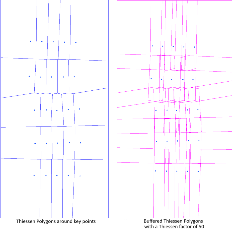
- Classic: Creates constraining polygons for the input images using PCI traditional algorithm that was developed for aerial images, that are approximately square and contain a lot of overlap. You can adjust the option by specifying a value for the Factor. In this case Factor represents the Theissen Factor. If you do not specify a value, the default value of 50 is applied.
- Strips: Create one constraint polygon for each input image using PCI algorithm that was developed for projects that have a clear pattern of strips, such as often seen with ADS data. Images must be of similar size and align in at least one direction from, for instance, aerial flight lines or satellite swaths. Cutline-constraining polygons is generated for each image based on where it and its neighbors have actual data. This method first tries to group the images in rows or columns, and chooses the strips with the most consistent distance between images. It then removes the overlap between images in each strip using, at most, two neighboring images. Finally overlap is remove between the different strips leaving a constraining polygon. The extents of the polygons can be manipulated by specifying a value for the overlap Factor. If you do not specify a value, the default value of 20 is applied.
- No: Does not apply constraint polygons.
You can adjust the effect of Auto Constrain by specifying an appropriate percentage value for Factor.
When a constraining layer is specified for Cutline Method Extra Options, do not use Auto Constrain; that is, select No.
Factor
The Factor is a percentage by which to adjust the effect of the Auto Constrain option.
This is a value between 1 and 100, with larger values causing more overlap between the generated constraint polygons; that is, the cutlines is less constrained.
Simplify Cutlines
Selected by default, this check box causes the module to simplify the cutlines for the mosaic. Simplification is to remove unsuitable vertices from the cutline shapes computed initially.
You can use this parameter in conjunction with Simplification Level to set the degree of simplification you want.
Simplification Level
Available when the Simplify Cutlines check box is selected, you can set the level of simplification you want to use.
When the Simpify Cutlines check box is clear, no simplification level is applied. When the check box is selected, a default value of 1.75 for Simplification Level is applied; otherwise, the value you specify is applied.
To create cutlines from all of the vertices computed initially, enter a value of 0. A number greater than zero increases the amount of vector reduction; the cutlines will have fewer vertices. Generally, a value of n results in 1/n of the vertices being computed. For example, a value of 2 results in approximately one half of the vertices.
Global Cutline Avoidance Mask File
The file that, in conjunction with Global Cutline Avoidance Mask Layer and Global Cutline Avoidance Mask Segment, can be used to identify common regions in all source images to omit from cutline calculations. When a global cutline-avoidance mask is used, the image pixels in the masked regions are excluded from the cutline calculations wherever possible; if there is no better area in which to place a cutline, the cutline passes through the masked region.
When you specify a value for this parameter, you must also specify a value for Global Cutline Avoidance Mask Layer.
Global Cutline Avoidance Mask Layer
The layer in the file specified for Global Cutline Avoidance Mask File to use as the global cutline-avoidance mask. When no value is specified for Global Cutline Avoidance Mask File, this parameter is ignored.
Global cutline-avoidance masks are used to restrict specific areas from cutline calculations; for example, to avoid cutlines crossing through buildings. When a global cutline-avoidance mask is used, the image pixels in the masked regions are excluded from the cutline calculations wherever possible; if there is no better area in which to place a cutline, the cutline passes through the masked region. A global cutline-avoidance mask applies to all source images that intersect the global mask layer.
- Last Vector: Sets the last-created vector segment in the file specified for Global Cutline Avoidance Mask File as the global cutline-avoidance mask layer.
- Last Bitmap: Sets the last-created bitmap segment in file specified for Global Cutline Avoidance Mask File as the global cutline-avoidance mask layer.
- Specific Segment: Defines a specific segment in the file specified for Global Cutline Avoidance Mask File as the global cutline-avoidance mask layer. When you select this option, you must specify a value for Global Cutline Avoidance Mask Segment.
Global Cutline Avoidance Mask Segment
When Specific Segment is selected for Global Cutline Avoidance Mask Layer, this parameter specifies the number of the segment that contains polygons or bitmaps to use to mask pixels to avoid when calculating cutlines.
Area of Interest File
A file that contains a single vector layer that defines the area to which the output mosaic is clipped.
The vector layer can contain one or more polygons.
Crop Tiles to AOI
Selected by default, this check box controls whether to crop the tiles to the area of interest (AOI) during processing.
Tile Base Name
The base name for file names of all tiles created during the mosaicking process.
Tile Specification
The tiling scheme to use for the output mosaic.
- Single Tile: Generates the output mosaic as a single tile.
- Vector: Use when you have an existing vector-polygon layer that contains the tile definitions you want to use for the mosaic. When you select this option, you can add options for it with Tile File, Segment Number, Field Name, and Buffer Distance, respectively.
- Dimensions: Creates tiles of a specific size. When you select this option, you can add options for it with Tile Height and Tile Width, respectively. When using this specification, the TileID values of the output tiles is generated using the convention <column_number>_<row_number>. For example, the upper-left tile always has a TileID of "1_1", the one immediately below is "1_2", and so on.
- Script File: Use when you have a text file that defines the coordinates of each tile you want to create. When you select this option, you can add options for it with Tile File.
Height
The height of the mosaic tile, in pixels.The union of the extents of all of the source images is divided into a series of evenly sized and abutting rectangular tiles with the specified dimension.
Only tiles that actually intersect at least one of the source images is present in the output. The tiles at the far right and on the far bottom may overhang the extents of the source images. This is done to ensure that all tiles have the same dimensions.
TileID values are generated using the convention <column_number>_<row_number>. For example, the upper-left tile always has a TileID of "1_1", while the one immediately below it is "1_2", and so on.
For example:
10000
Width
The width of the mosaic tile, in pixels.The union of the extents of all of the source images is divided into a series of evenly sized and abutting rectangular tiles with the specified dimension.
Only tiles that actually intersect at least one of the source images is present in the output. The tiles at the far right and on the far bottom may overhang the extents of the source images. This is done to ensure that all tiles have the same dimensions.
TileID values are generated using the convention <column_number>_<row_number>. For example, the upper-left tile always has a TileID of "1_1", while the one immediately below it is "1_2", and so on.
For example:
10000
Vertical Overlap
The vertical overlap of each tile, in pixels.
Horizontal Overlap
The horizontal overlap of each tile, in pixels.
Tile File
The name of the text file containing the tile-definition layer.Each line in the text file contains five elements separated by spaces: the first two define the upper-left coordinate in the x and y dimension, respectively. The next two define the lower-right coordinate in the x and y dimensions, respectively. The last one specifies the output file name of the tile. If the file name includes an extension, the extension is removed when the value is stored as the 'TileID' attribute in the tile-definition polygon. If the file name includes a path, the entire path is transferred and appended to the output folder.
- RASEXT: Raster extents
- GEOEXT: Geocoded extents
- LNGLATEX: Longitude and latitude extents
- RASOFFSZ: Raster offset and size
- GEOOFFSZ: Geocoded offset and size
The RASEXT and RASOFFSZ coordinate types make use of pixel/line raster, as defined by the union of the extents of all input source images. If a coordinate type is not specified, it is assumed to be GEOEXT. For example:
Segment Number
In the tile file you specified, the number of the vector segment to use. If no segment number is specified, the last segment in the specified tile file is used.Field Name
Name of the field (attribute) that has unique identifiers for each tile. The module uses the values in the field to form the names of the mosaic tile files. If no field name is specified, the attribute ShapeID is used.Coordinate Type
When Tile Specification is Script File, the type of coordinates in the script.
- Geocoded Extents
- Geocoded Offset & Size
- Long/Lat Extents
- Raster Extents
- Raster Offset & Size
Tile Position Transformation
With this parameter you can define a grid where each top-left corner of a tile is aligned to one of the vertices in the grid.
- CORNER: indicates that the values are relative to the upper-left corner of the first pixel in the output tile
- CENTER: indicates that the values are relative to the center of the first pixel
- Stride_X
- Stride_Y
- Ref_X
- Ref_Y
These values define the position of the corner or center in the raster grid.
Of the four values, only Stride_X is required. If not specified, Stride_Y defaults to the Stride_X value, and Ref_X and Ref_Y default to zero.
In the following example, the upper-left corner of the upper-left pixel of each tile is an even 20-meter multiple from the reference point (432345.000, 5438882.000). Depending on the distance of the tile from that point, its upper-left corner coordinate could be 432345.000, 432045.000, or any other multiple, but is never 432346.000 or 432355.000.
Example:
"CORNER, 20, 20, 432345.000, 5438882.000"
If specified, this parameter is applied in all scenarios, whether the image-corner coordinates come from the input file (MFILE), ULX and ULY, or through automatic computation.
Blend Width
The perpendicular distance from the cutlines over which image blending occurs.
Image blending is to average the gray value of each pixel in the blending strip along a cutline from both overlapping input images. If no value is specified for this parameter, no blending is performed.
Create Source Map
Select this check box to create a source map on output along with the mosaic.
A source map is a polygon layer created and stored in a separate file, which contains an attribute that identifies the predominant source input image used for each pixel in the output mosaic. As images are added to the mosaic, the source image is recorded in a separate raster, which is converted to a polygon layer at the end of the process.
- SourceID: a text field that contains the SourceID of the source image.
- SourceFile: a text field that includes the full GDB string including path to the source input image.
- Z-order: an integer field that records the z-order of the predominate source image. The word "predominant" is used because, in the case of blending along cutlines, the source scene which had the largest contribution is the one indicated.
The source map layer is created in a file with the same name as the output mosaic file(s), but with _SourceMap.pix appended to it.
Existing Tile Rule
Select an action to perform when an output tile already exists.
Available options are:
Skip: No change is made to the existing tile and no new processing is performed. This option is useful when you do not want to modify your existing mosaic output.
Note: When an existing tile is skipped, it is not checked to see if it is empty. The tile is never deleted, regardless of the value of Delete Empty Tile.- Regenerate: Any existing tile is deleted, and then a new tile created. Unlike Skip or Update, the output is in the same projection and extents as the new polygon-tile definition.
- Update: An existing tile is updated with any new information. The existing information is not overwritten; rather, the file is appended with any new information resulting from the mosaicking. Any existing georeferencing is safeguarded.
Delete Empty Tiles
Select whether to delete empty tiles. A tile is considered to be empty if all pixels in it have the value defined as NoData.